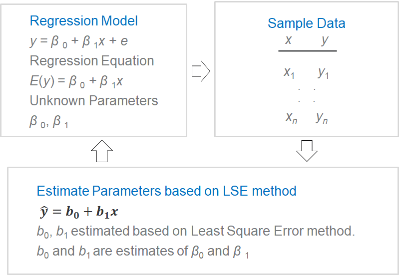
Exhibit 34.26 Estimation process.
The approach to estimating the parameters for a regression equation is outlined in
Exhibit 34.26. The intercept and coefficient estimates are based on the Least Squares Error
(LSE) method where the criterion is to minimize the sum of the squared error (SSE) (actual – predicted):
$$ min\sum(y_i-\hat y_i)^2 $$
yi: observed value.
ŷi: estimated value.
In the case of simple linear regression:
$$ SSE = \sum_{i=1}^n (y_i - \hat y_i )^2 = \sum_{i=1}^n [y_i - (b_0 + b_1 x_i)]^2 $$
Via differentiation we can obtain the estimate for the regression coefficient:
$$b_1= \frac{\sum(x_i-\bar x)(y_i-\bar y)}{\sum(x_i - \bar x)^2}=\frac{SS_{xy}}{SS_{xx}}$$
And, b0, the intercept:
$$ b_0=\bar y - b_1 \bar x $$
As with simple regression, estimates for multiple linear regression are based on the
LSE method. The parameters b1, b2, b3 etc. are called partial
regression coefficients. They reveal the importance of their respective predictor variables,
in driving the response variable.
Note: The b-coefficients, which represent the partial contributions of
each x-variable, may not necessarily agree in relative magnitude or even in sign with
the bivariate correlation between each x-variable and the dependent variable, y.
Regression coefficients vary with measurement scales. If we standardize (i.e., subtract
the mean and divide by the standard deviation) y as well as x1,
x2, x3, the resulting equation is scale-invariant:
$$ z_y = b_0^* + b_1^* × z_{x1} + b_2^* × z_{x2} + b_3^* × z_{x3}\, …$$