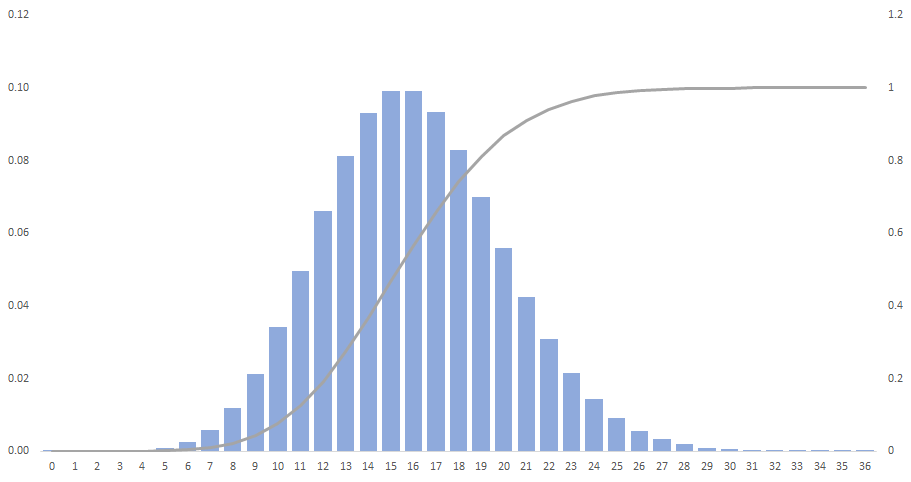
Exhibit 34.11 Poisson distribution, λ = 16.
Poisson distribution (Exhibit 33.10) expresses the probability of a given number
of events occurring in a fixed interval of time or space, if these events occur with a known constant
rate and independently of the time since the last event.
The distribution is useful for modelling number of occurrences of an event over a
period of time, for instances:
- Customers arriving at an ATM.
- Shoppers arriving at a retail outlet.
- Calls on a hotline.
- Fatal accidents.
Properties:
- Probability of an occurrence is the same for any two intervals of equal length.
- Occurrences in non‐overlapping intervals are independent of one another.
A random variable X is said to be a Poisson random variable with parameter λ (> 0) if it has the
probability function:
$$P(X=i)=\frac{e^{-λ} λ^i}{i!},\,for \,i \,(occurances)=0,1,2…$$
$$P(X=0)=\frac{e^{-λ} λ^0}{0!}= e^{-λ}$$
$$P(X=1)=\frac{e^{-λ} λ^1}{1!}= λe^{-λ}$$
It can be shown that:
$$Mean \,E(X) = λ$$
$$Variance \,Var (X) = λ$$
Thus, parameter λ can be interpreted as the average number of occurrences per unit time
or space.
Example 1: Patients arrive at the A & E of a hospital at the average rate of 6 per
hour on weekend evenings. What is the probability of 4 arrivals in 30 minutes on a weekend evening?
$$λ = \text{3 per 30 minutes}$$
$$P(X=4)=\frac{e^{-3} 3^4}{4!}=0.168 = 16.8 \% $$
Example 2: Customers arrive at a row of ATMs at the average rate of 96 per hour
during peak hours (weekday noon). What is the probability of 20 or more arrivals over 10 minutes on a
weekday afternoon?
λ = 16 per 10 minutes. The Poisson distribution for λ = 16 is depicted in Exhibit
34.11.
$$P(X≥20)=1-P(X<=19)= 1-\sum_{i=0}^{19}\frac{e^{-16}16^i}{i!}=1-0.812=0.188$$
There is 18.8% likelihood that 20 or more customers will arrive at the row of ATMs, over
any 10-minute interval, on a weekday afternoon.
Note: Excel’s Poisson distribution function is POISSON.DIST (x, λ, cumulative).


