
-
Basic Statistics
Basic Statistics
Probability Theory
Mutually Exclusive Events and Overlapping Events
Objective and Subjective Probabilities
Conditional (Posterior) Probability
Independent Events
Law of Total Probabilities
Bayes Theorem
Discrete Probability Distribution
Binomial Distribution
Poisson Distribution
Relationship between Variables
Covariance and Correlation
Joint Probability Distribution
Sum of Random Variables
Correlation and Causation
Simpson’s Paradox
Continuous Probability Distributions
Uniform Distribution
Exponential Distribution
Normal Distribution
Standard Normal Distribution
Approximating Binomial with Normal
t-test
Hypothesis Testing
Type I and Type II Errors
Statistical Significance and Practical Significance
Hypothesis Testing Process
One-Tailed — Known Standard Deviation
Two-tailed — Known Standard Deviation
One-Tailed — Unknown Standard Deviation
Paired t-test
ANOVA
Chi-Square (χ2)
Regression
Simple Linear and Multiple Linear Regression
Least Squares Error Estimation
Overview
Sample Size
Choice of Variables
Assumptions
Normality
Linearity
Dummy Variables
Interaction Effects
Variable Selection Methods
Issues with Variables
Multicollinearity
Outliers and Influential Observations
Coefficient of Determination (R2)
Adjusted R2
F-ratio: Overall Model
t-test: Coefficients
Goodness-of-fit
Validation
Process
Factor Analysis
- Basic Statistics
- Sampling
- Marketing mix Modelling
Coronavirus — What the metrics do not reveal?
Coronavirus — Determining death rate
- Marketing Education
- Is Marketing Education Fluffy and Weak?
- How to Choose the Right Marketing Simulator
- Self-Learners: Experiential Learning to Adapt to the New Age of Marketing
- Negotiation Skills Training for Retailers, Marketers, Trade Marketers and Category Managers
- Simulators becoming essential Training Platforms
- What they SHOULD TEACH at Business Schools
- Experiential Learning through Marketing Simulators
-
MarketingMind
Basic Statistics
Basic Statistics
Probability Theory
Mutually Exclusive Events and Overlapping Events
Objective and Subjective Probabilities
Conditional (Posterior) Probability
Independent Events
Law of Total Probabilities
Bayes Theorem
Discrete Probability Distribution
Binomial Distribution
Poisson Distribution
Relationship between Variables
Covariance and Correlation
Joint Probability Distribution
Sum of Random Variables
Correlation and Causation
Simpson’s Paradox
Continuous Probability Distributions
Uniform Distribution
Exponential Distribution
Normal Distribution
Standard Normal Distribution
Approximating Binomial with Normal
t-test
Hypothesis Testing
Type I and Type II Errors
Statistical Significance and Practical Significance
Hypothesis Testing Process
One-Tailed — Known Standard Deviation
Two-tailed — Known Standard Deviation
One-Tailed — Unknown Standard Deviation
Paired t-test
ANOVA
Chi-Square (χ2)
Regression
Simple Linear and Multiple Linear Regression
Least Squares Error Estimation
Overview
Sample Size
Choice of Variables
Assumptions
Normality
Linearity
Dummy Variables
Interaction Effects
Variable Selection Methods
Issues with Variables
Multicollinearity
Outliers and Influential Observations
Coefficient of Determination (R2)
Adjusted R2
F-ratio: Overall Model
t-test: Coefficients
Goodness-of-fit
Validation
Process
Factor Analysis
- Basic Statistics
- Sampling
- Marketing mix Modelling
Coronavirus — What the metrics do not reveal?
Coronavirus — Determining death rate
- Marketing Education
- Is Marketing Education Fluffy and Weak?
- How to Choose the Right Marketing Simulator
- Self-Learners: Experiential Learning to Adapt to the New Age of Marketing
- Negotiation Skills Training for Retailers, Marketers, Trade Marketers and Category Managers
- Simulators becoming essential Training Platforms
- What they SHOULD TEACH at Business Schools
- Experiential Learning through Marketing Simulators
Hypothesis Testing
A hypothesis test examines two mutually exclusive claims about a parameter to determine which is best supported by the sample data. The parameter is usually the mean or proportion of some population variable of importance to the marketer.
The null hypothesis (H0) is the status quo or the default position that there is no relationship or no difference. The alternative or research hypothesis (HA) is the opposite of the null. It represents the relationship or difference.
Type I and Type II Errors
The conclusion of the hypothesis test can be right or wrong. Erroneous conclusions are classified as Type I or Type II.
Type I error or false positive occurs when the null hypothesis is rejected, even though it is actually true. There is no difference between the groups, contrary to the conclusion that a significant difference exists.
Type II error or false negative occurs when the null hypothesis is accepted, though it is actually false. The conclusion that there is no difference is incorrect.
An oft quoted example is of the jury system where the defendant is “innocent until proven guilty” (H0 = “not guilty”, HA = “guilty”). The jury’s decision whether the defendant is not guilty (accept H0), or guilty (reject H0), may be either right or wrong. Convicting the guilty or acquitting the innocent are correct decisions. However, convicting an innocent person is a Type I error, while acquitting a guilty person is a Type II error.
Though one type of error may sometimes be worse than the other, neither is desirable. Researchers and analysts contain the error rates by collecting more data or greater evidence, and by establishing decision norms or standards.
A trade-off however is required because adjusting the norm to reduce type I error results in the increase in type II error, and vice versa. Expressed in terms of the probability of making an error, the standards are summarized in Exhibit 34.20:
| Truth | ||
| No Difference (H0 true) | Difference (H0 false) | |
| Accept H0 | 1 – α | β: Type II |
| Reject H0 | α: Type I | 1 – β: Power |
Exhibit 34.20 Probability of type I error (α), probability of type II error (β), and power (1- β), the probability of correctly rejecting the null hypothesis.
α: Probability of making a Type I error, also referred to as the significance level, is usually set at 0.05 or 5%, i.e., type I error occurs 5% of the time.
β: Probability of making a Type II error.
1 – β: Called power, is the probability of correctly rejecting the null hypothesis.
Power is the probability of correctly rejecting the null hypothesis, i.e., correctly concluding there was a difference. This usually relates to the objective of the study.
Power is dependent on three factors:
- Type I error (α) or significance level: Power decreases with decrease in significance level. The norm for quantitative studies is α = 5%.
- Effect size (Δ): The magnitude of the “signal”, or the amount of difference between the parameters of interest. This is specified in terms of standard deviations, i.e., Δ=1 pertains to a difference of 1 standard deviation.
- Sample size: Power increases with sample size. While very small samples make statistical tests overly sensitive, very large samples make them insensitive. With excessively large samples, even very small effects can be statistically significant, which raises the issue of practical significance vs. statistical significance.
Power is usually set at 0.8 or 80%, which makes β (type II error) equal to 0.2.
Since both α and power (or β) are typically set according to norms, the size of a sample is essentially a function of the effect size, or the detectable difference. This is discussed further in Section Sample Size — Comparative Studies, in Chapter Sampling.
Statistical Significance and Practical Significance
From the viewpoint of taking decisions, the distinction between statistical significance and practical or market significance must be clearly understood.
Take for example the results of a product validation test (e.g., BASES) reveal, with statistical significance, that a new formulation is likely to increase a brand’s sales by a million dollars. If the gain in sales is too small to offset the costs of introducing the new variant, then the increase is not significant enough to justify the launch of the variant.
In another example, pertaining to a retail bank, a number of initiatives targeting high-value customers, may have resulted in the reported increase in their customer satisfaction rating from 3.0 to 3.5, on a 5 point-scale. This increase suggests that the initiatives had an impact on customer satisfaction. But, if the p-value for the data is 0.1, in that case the result is not statistically significant at the usual level (α=0.05). There is a 10% chance that the difference is merely resulting from sampling error.
If the sample size is increased so that the results are statistically significant, that would increase the level of confidence that the difference is “real” and would justify the introduction of the new initiatives.
Hypothesis Testing Process
Hypothesis tests are classified as one-tailed or two-tailed tests. The one-tailed test specifies the direction of the difference, i.e., the null hypothesis, H0, is expressed in terms of the equation parameter ≥ something, or parameter ≤ something.
For instance, in a before and after advertisement screening test, if the ad is expected to improve consumers’ disposition to try a new brand, then the hypothesis may be phrased as follows:
H0, null hypothesis: Dafter ≤ Dbefore
HA, research hypothesis: Dafter > Dbefore
Where D is the disposition to try the product, expressed as the proportion of respondents claiming they will purchase the brand.
If the direction of the difference is not known, a two-tailed test is applied. For instance, if for the same test, the marketer is interested in knowing whether there is a difference between men and women, in their disposition to buy the brand, the hypothesis becomes:
H0, null hypothesis: Dmale = Dfemale
HA, research hypothesis: Dmale ≠ Dfemale
The standard process for hypothesis testing comprises the following steps:
- H0, HA: State the null and alternative hypothesis.
- α: Set the level of significance, i.e., the type I error. For most research studies this is set at 5%.
- Test statistic: Compute the test statistic. Depending on the characteristics of the test this is either the z-score (standard score), the t-value, or the f-ratio.
- p-value: Obtain the p-value by referencing test statistic in the relevant distribution table. The normal distribution is used for referencing the z-score, t distribution for the t-value and the f distribution for the f-ratio.
- Test: Accept the research hypothesis HA (reject H0) if p-value < α.
Each of the test statistics is essentially a signal-to-noise ratio, where the signal is the relationship of interest (for instance, the difference in group means), and noise is a measure of variability of groups.
If a measurement scale outcome variable has little variability it will be easier to detect change than if it has a lot of variability (see Exhibit 34.19). So, sample size is a function of variability.
A z-score (z) indicates how many standard deviations the sample mean is from the population mean.
$$ z = \frac{\bar x-μ}{s/\sqrt n} $$Where x̄ is the sample mean, μ is the population mean, and σ=s/√n is the sample standard deviation (refer CLT), and s is the standard deviation of the population.
Details of the t-test are provided in the section t-test, and the f-ratio is covered in the section ANOVA.
Note: The data analysis add-in in excel provides an easy-to-use facility to conduct hypothesis z, t and f tests. P-value calculators are also available online, for instance, at this Social Science Statistics webpage.
One-Tailed — Known Mean and Standard Deviation
For one-tailed, known mean and standard deviation tests the test statistic to use is the z-score.
Example: A range of initiatives, including increases in excise duty, constraints on pack sizes, and restrictions on distribution channels, were implemented with the aim of reducing cigarette consumption. The government set a target of decreasing consumption to below 120 sticks per smoker per month.
To evaluate the effectiveness of these measures, a study was conducted, involving 100 smokers. The findings revealed that, on average, each smoker consumed 28 sticks per week, amounting to 112 sticks per month.
To provide further context, an earlier large-scale consumption study estimated the standard deviation of cigarette consumption to be 40 sticks per month.
Based on these findings, can we conclude whether the government achieved its target?
H0: μ ≥120
HA: μ<120
α = 5%
$$ z = \frac{\bar x-μ}{s/\sqrt n} = \frac{112-120}{40/10} = -2.0 $$p-value = 0.023 < α = 0.05
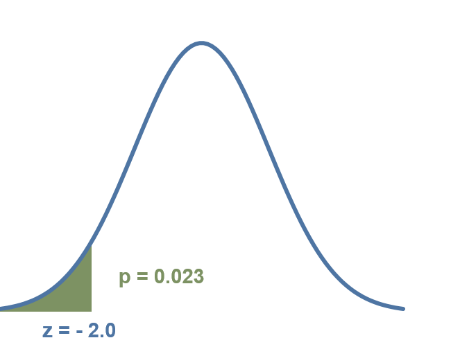
Exhibit 34.21 Probability that the sample average consumption of cigarettes is less than 120 is 0.023 or 2.3%.
The p-value, as depicted in Exhibit 34.21, indicates that the probability of obtaining a z-score of −2.0 or lower is 0.023. Using this information, we can infer that there is a 97.7% probability (1 − 0.023) that the government’s initiatives have effectively achieved the objective of reducing cigarette consumption to less than 120 sticks per month.
The null hypothesis is rejected because the p-value, 0.023 (2.3%), is less than α, 5%.
Note: A p-value from z-score calculator is provided on this webpage.
Two-tailed — Known Mean and Standard Deviation
Two-tailed tests with known mean and standard deviation also use the z-score statistic. In such cases, the z-score can be used in conjunction with the normal distribution, provided that the population’s standard deviation is known.
Example: The mean weight of fresh recruits into the army was reported to be 65.8 kg last year. This year, a sample of 200 recruits was taken, and the mean weight was found to be 66.2 kg. Assuming the population standard deviation is 3.2 kg, at 0.05 significance level, can we conclude that the mean weight has changed since last year?
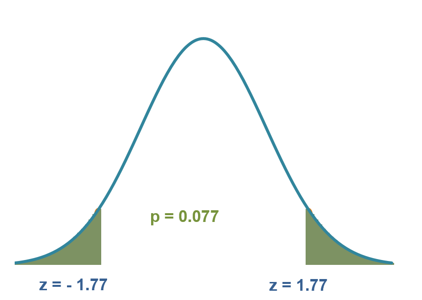
Exhibit 34.22 If the actual mean was 65.8 kg, there is a 7.7% probability that the sampled recruits would weigh ≥ 66.2 kg or ≤ 65.4 kg.
H0: μ=65.8
HA: μ≠65.8
α = 5%
$$ z = \frac{\bar x-μ}{s/\sqrt n} = \frac{66.2-65.8}{3.2/14.14} = 1.77 $$p-value = 0.077 > α = 0.05
The p-value of 0.077 (7.7%), obtained from normal distribution (Exhibit 34.22) for z = 1.77, is not significant for the given level of 5%.
If the actual mean was 65.8 kg, there is a 7.7% probability that the sampled recruits would weigh ≥ 66.2 kg or ≤ 65.4 kg. Since this probability is higher than the significance level of 5%, the null hypothesis is not rejected. We cannot conclude with 95% certainty that the new recruits differ in weight from those recruited last year.
One-Tailed — Unknown Standard Deviation
In cases where the population standard deviation is not known, t-value is used as the test statistic for one-tailed tests. (Refer section t-test for details on the test and the t-value).
Example: To assess whether the proportions of surfactant in the detergent packs are correct, a study was conducted by technicians from a contracted lab. The study involved examining samples from 80 packs. According to the specifications, the packs should contain an average of 15% surfactant.
The findings from the sample indicate that the average surfactant composition in the sampled packs is 14.7 grams per 100 grams of detergent, with a standard deviation of 1.2 grams. Based on these findings, can we infer that the packs contain less than the specified level of surfactant?
H0: μ ≥ 15 gm per 100 gm of detergent
HA: μ < 15 gm per 100 gm of detergent
α = 5%
$$ t = \frac{\bar x-μ_0}{σ/\sqrt n} = \frac{14.7-15}{1.2/8.94} = -2.24 $$Degrees of freedom = 79.
p-value = 0.014.
The probability of obtaining a t-value of −2.24 or lower, when sampling 80 packs from the population, has been determined to be 0.014 or 1.4%. This probability is lower than the significance level α of 5%. In other words, if the average surfactant concentration is assumed to be 15%, the probability that our sample would have an average of 14.7% or less is only 0.014 (1.4%). Based on this analysis, the null hypothesis is rejected, indicating that the data suggests that the manufacturer is not meeting the specified concentration of 15%.
Note: A p-value from t-value calculator is provided on this webpage.
Paired t-test
Paired group test with unknown standard deviation is essentially the same as a single sample t-test. The paired values are reduced to a single series by computing the difference between the two sets.
Example: In advertising copy tests, purchase intent is gauged through pre-post exposure measurement of respondents’ disposition to buy or try a product. The metric, x, is usually the top-2 box rating (“very likely to buy”, “likely to buy”). The paired values (xbefore, xafter) are reduced to a single set of values (y) by computing the difference: y = xafter – xbefore. HA: μ > 0, i.e., exposure to the advert is expected to improve disposition to try the product.
Example: Sequential monadic tests are frequently used for product testing. The respondents try one product and rate it, move to another product and rate it, and then compare the two. A paired t-test may be used to determine whether an improved formulation is rated higher on an attribute. HA: μ > 0, i.e., new product expected to be rated higher.
The remaining steps are the same as that for a one-tailed, single sample t-test.
Comparison test for two groups of unknown standard deviation also requires use of the t-test, since the population’s standard deviation is not known.
Example: A study was conducted to examine the consumption of coffee by office workers. The statistics for the men and women sampled in this study are given below.
Men: Sample size nM=440, mean x̄M =46.5 cups per month, standard deviation sM=36.3.
Women: Sample size nW=360, mean x̄W=35.1 cups per month, standard deviation sW=20.6.
There is a difference of 11.4 cups per month in coffee consumption between men and women. Is this difference resulting from sampling error, or do men consume significantly more coffee than women?
H0: μM – μW < 0
HA: μM – μW > 0
α = 0.05
Standard deviation:
$$ σ_{\bar x_M-\bar x_M} = \sqrt {\frac{s_M^2}{n_M} + \frac{s_W^2}{n_W}} = \sqrt {\frac{36.3×36.3}{440} + \frac{20.6×20.6}{360}} = 2.04 $$ $$ t=\frac{\bar x_M-\bar x_W}{σ_{\bar x_M - \bar x_W}} =\frac {46.5-35.1}{2.04}=5.58 $$ $$ degrees\;of\; freedom\; (df) = \frac {\left(\frac {s_M^2}{n_M} + \frac {s_W^2}{n_W}\right)^2} {\frac{(s_M^2/n_M)^2}{n_M-1}+\frac {(s_W^2/n_W)^2}{n_W-1}} = 716.8 $$p-value = 0.00001 obtained from t distribution.
The probability of obtaining a t-value of 5.58 or higher with 717 degrees of freedom, when sampling 440 men and 360 women is very low (0.00001 << α = 0.05). More specifically, if women were consuming as much coffee as men, the chance that the sample differences would average 11.4 or more cups per month is only 0.00001. The null hypothesis is rejected. The data strongly suggests that women consumers consume less coffee than men.
Previous Next
Use the Search Bar to find content on MarketingMind.


Contact | Privacy Statement | Disclaimer: Opinions and views expressed on www.ashokcharan.com are the author’s personal views, and do not represent the official views of the National University of Singapore (NUS) or the NUS Business School | © Copyright 2013-2026 www.ashokcharan.com. All Rights Reserved.