Customised Sentiment Analysis

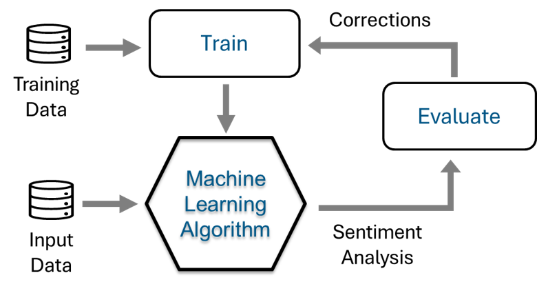
Exhibit 25.28   Customized Sentiment Analysis: The machine learning algorithm is trained using labeled training data.

Pre-trained classifiers like VADER are effective for general applications but may not suit domain-specific requirements. For specialised needs, classifiers should be trained using customised and verified labelled datasets.

Steps for Customised Sentiment Analysis:

• Label Dataset: Carefully label the dataset to ensure it meets the analysis objectives.
• Construct Training and Test Sets: Divide the dataset into training and test sets for model evaluation.
• Model Creation: Naive Bayes is one example of a model used for creating custom Sentiment Analysis classifiers.

Exhibit 25.29 demonstrates the implementation of custom sentiment analysis using Python with a dataset of tweets (tweets.csv. The process involves the following steps:

1. Data cleaning and pre-processing: Tokenizing and cleaning the tweets in the raw data file.
2. Sentiment analysis: Sentiment analysis of the original tweets in the raw data.
3. Construct training and test datasets: Prepare training and testing datasets by selecting the first 45 rows for training and rows 46 to 70 for testing.
4. Naive Bayes classification: Implement a Naive Bayes classification model for text data using the TF-IDF (Term Frequency-Inverse Document Frequency) representation of the text.
5. Model validation: Evaluate the Naive Bayes model using a classification report and confusion matrix on test data, and perform 10-fold cross-validation on training data to compute the cross-validation accuracy.

(3) Construct Training and Test Datasets

This section of the Python code performs several key tasks, starting with serializing a DataFrame (df1) using the pd.to_pickle() function. The DataFrame is saved in a file named tagged.pickle, which stores the data in a Python-specific binary format, enabling both serialization and deserialization of the DataFrame. The serialized data is then reloaded into the program using pd.read_pickle() to create a new dataset.

Next, the code defines three classes—'pos', 'neu', and 'neg'—that are likely used for categorizing the data. It proceeds to construct training and test datasets from the dataset DataFrame. Specifically, the first 45 rows of the 'tokenized_and_cleaned' column are extracted as train_data, and the corresponding labels from the 'Labels' column are assigned to train_labels. Similarly, the code selects rows 46 to 70 for test_data and test_labels to be used for testing.

Before proceeding with the training process, the train_data is converted into a list of strings by applying the join function to concatenate tokenized words into full sentences. The first five entries of this training dataset are printed for inspection using pprint(). The same concatenation process is applied to the test_data, preparing it for later use in evaluating the model.

(4) Naive Bayes Classification

This Python code implements a Naive Bayes classification model using TF-IDF (Term Frequency-Inverse Document Frequency) representation for text data. Vectorization is the process of transforming textual data into a numerical format that can be understood by machine learning algorithms. Each word or phrase in the text is converted into a feature vector, where each element represents the importance or relevance of that term in the document.

The process begins by importing necessary libraries: TfidfVectorizer from sklearn.feature_extraction.text to convert the text into numerical features based on TF-IDF values, and MultinomialNB from sklearn.naive_bayes to implement the Naive Bayes classifier, which is commonly used for text classification.

The text data is first vectorized using TfidfVectorizer, where specific parameters are set to fine-tune the vectorization process. For example, min_df=5 ignores words that appear in fewer than 5 documents, while max_df=0.8 excludes words that appear in more than 80% of the documents, as these are likely too common to be useful for classification. The option sublinear_tf=True applies sublinear scaling to term frequency, and use_idf=True ensures that inverse document frequency (IDF) is applied to reduce the importance of frequently occurring words.

The vectorizer is then fit to the training data (train_data), transforming it into a TF-IDF matrix where each row corresponds to a document, and each column represents a feature (a word). This transformation is also applied to the test data (test_data) using the same vectorizer, ensuring that both training and test data share a consistent feature set.

Next, the Naive Bayes classifier is created using MultinomialNB(). The model is trained on the TF-IDF vectors of the training data using the nb.fit() method, which takes the transformed training data (train_vectors) and their corresponding labels (train_labels) as inputs. After training, the model’s accuracy is evaluated on the test data (test_vectors) by comparing the predicted labels with the actual test labels (test_labels). This is done using the .score() method, which returns the accuracy of the model on the test data.

(5) Model Validation

The code begins by importing necessary libraries to evaluate the Naive Bayes model. The classification_report, confusion_matrix, and accuracy_score functions from sklearn.metrics are used to assess the model’s performance, while cross_val_predict from sklearn.model_selection is employed to perform cross-validation on the training data.

To evaluate the model on the test data, the trained Naive Bayes classifier (nb) predicts labels for the test data (test_vectors). A classification report is then generated by comparing the predicted labels with the true test labels (test_labels). This report includes key metrics such as precision, recall, F1-score, and support for each class, which provide detailed insights into the model’s performance across different categories. Additionally, a confusion matrix is printed, showing the number of true positives (TP), true negatives (TN), false positives (FP), and false negatives (FN). This matrix offers a visual breakdown of how accurately the model classified the test data.

The code also performs 10-fold cross-validation on the training data (train_vectors and train_labels). In this process, the dataset is divided into 10 folds, and the model is trained on 9 of these folds while being tested on the remaining fold. This procedure is repeated 10 times, generating cross-validation predictions for the entire training set using the cross_val_predict function. The overall accuracy of the model during cross-validation is then calculated by comparing the predicted labels with the true training labels, and the cross-validation accuracy is printed as a percentage, reflecting the model’s average performance across all folds.

Data Cleaning and Pre-processing

Copy Code

import nltk
from nltk.tokenize import TweetTokenizer
from nltk.corpus import stopwords
import string
import pandas as pd
nltk.download('stopwords')

# df: Read tweets and load them into the dataframe df
df = pd.read_csv("data/tweets.csv")

# tokens: Tokenize and store in the 'tokens' column
df['tokens'] = df['text'].apply(TweetTokenizer().tokenize)

# stopwords_removed: Remove stopwords
stopwords_vocabulary = stopwords.words('english')
df['stopwords_removed'] = df['tokens'].apply(lambda x: [i for i in x if i.lower() not in stopwords_vocabulary])

# punctuations_removed: Removing punctuations
punctuations = list(string.punctuation)
df['punctuations_removed'] = df['stopwords_removed'].apply(lambda x: [i for i in x if i not in punctuations])

# digits_removed: Remove tokens beginning with a digit
df['digits_removed'] = df['punctuations_removed'].apply(lambda x: [i for i in x if i[0] not in list(string.digits)])

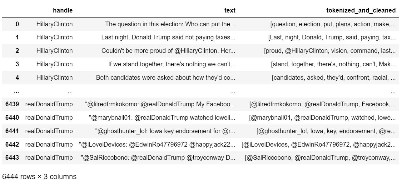
# tokenized_and_cleaned: Remove single character tokens
df['tokenized_and_cleaned'] = df['digits_removed'].apply(lambda x: [i for i in x if len(i) > 1])

print("tokenized_and_cleaned tweets")
df[['handle', 'text', 'tokenized_and_cleaned']] 

from pprint import pprint  # pretty print
from nltk.sentiment.vader import SentimentIntensityAnalyzer
sentiment = SentimentIntensityAnalyzer()

# Sentiment analysis of the original tweets in the text column of df
# sentiment: store polarity scores in a column 'sentiment' 
df['sentiment'] = df.text.apply(lambda x: sentiment.polarity_scores(x)['compound'])

# Labels: Tag the tweets as 'neg', neu' and 'pos'
df['Labels'] = ['neg' if x<0 else 'neu' if x==0 else 'pos' for x in df['sentiment']]
df1 = df[['tokenized_and_cleaned','Labels']]
print("Dataset df1:\n",df1.head(5))

Dataset df1:
                                tokenized_and_cleaned Labels
0  [question, election, put, plans, action, make,...    pos
1  [Last, night, Donald, Trump, said, paying, tax...    neu
2  [proud, @HillaryClinton, vision, command, last...    pos
3  [stand, together, there's, nothing, can't, Mak...    pos
4  [candidates, asked, they'd, confront, racial, ...    neg

# Serialize df1
'''
pd.to_pickle() function is used to serialize df1 into a pickle format and 
save it to file tagged.pickle. Pickle is a Python-specific binary format for 
serializing and deserializing Python object structures.
'''
pd.to_pickle(df1, "./tagged.pickle")
dataset  = pd.read_pickle('tagged.pickle')

classes = ['pos', 'neu', 'neg']

# Construct the Training and Test Datasets
# train data - use the data in the 1st 45 rows for training the classifier 
train_data = dataset['tokenized_and_cleaned'][0:45]
train_labels = dataset['Labels'][0:45]
      
# test data - use rows 46 to 70 for testing
test_data = dataset['tokenized_and_cleaned'][46:71]
test_labels = dataset['Labels'][46:71]

train_data = list(train_data.apply(' '.join))
print("Training Dataset [0:5]:")
pprint(train_data[0:5])
test_data = list(test_data.apply(' '.join))

Training Dataset [0:5]:
['question election put plans action make life better https://t.co/XreEY9OicG',
 'Last night Donald Trump said paying taxes smart know call Unpatriotic '
 'https://t.co/t0xmBfj7zF',
 "proud @HillaryClinton vision command last night's debate showed ready next "
 '@POTUS',
 "stand together there's nothing can't Make sure ready vote "
 'https://t.co/tTgeqxNqYm https://t.co/Q3Ymbb7UNy',
 "candidates asked they'd confront racial injustice one real answer "
 'https://t.co/sjnEokckis']

# Creating the model – Naive Bayes
'''
Implementing a Naive Bayes classification model for text data using the TF-IDF 
(Term Frequency-Inverse Document Frequency) representation of the text. 
'''

# To convert text into numerical features based on TF-IDF values.
from sklearn.feature_extraction.text import TfidfVectorizer

# Naive Bayes classifier used for text classification.
from sklearn.naive_bayes import MultinomialNB  

# Vectorizing the text:
'''
min_df=5: Ignore words that appear in fewer than 5 documents.

max_df=0.8: Ignore words that appear in more than 80% of the documents 
    (likely to be too common and not meaningful for classification).

sublinear_tf=True: Apply sublinear term frequency scaling, which replaces raw term 
    frequency with 1 + log(tf).
    
use_idf=True: Use inverse document frequency (IDF) to scale down the impact of 
    frequently occurring words in the corpus.
'''
vectorizer = TfidfVectorizer(min_df=5, max_df = 0.8, sublinear_tf=True, use_idf=True)

''' 
Fit the vectorizer to the training data (train_data) and transforms it into a 
TF-IDF matrix where each row represents a tweet, and each column represents a word.
'''
train_vectors = vectorizer.fit_transform(train_data)

''' 
Transform the test data (test_data) using the same vectorizer that was fit to the 
training data, ensuring consistency between training and test features.
'''
test_vectors = vectorizer.transform(test_data)

# Naive Bayes Classifier creates an instance of the Multinomial Naive Bayes classifier.
nb = MultinomialNB()

'''
nb.fit(train_vectors, train_labels): Trains the Naive Bayes model using the TF-IDF 
    vectors of the training data (train_vectors) and their corresponding labels 
    (train_labels).
    
.score(test_vectors, test_labels): After training, this evaluates the model on the 
    test data (test_vectors) and calculates the accuracy score by comparing the 
    predicted labels with the true labels (test_labels).
'''
nb.fit(train_vectors, train_labels).score(test_vectors, test_labels)

0.88

'''
Evaluation of the Naive Bayes Model:
    Evaluate the Naive Bayes model using a classification report and confusion 
    matrix on test data, and perform 10-fold cross-validation on training data 
    to compute the cross-validation accuracy.
'''

# Functions help evaluate the performance of a classification model.
from sklearn.metrics import classification_report, confusion_matrix, accuracy_score

# Function to cross-validate the training data, predicting labels for each fold.
from sklearn.model_selection import cross_val_predict

'''
nb.predict(test_vectors): Uses the trained Naive Bayes classifier (nb) to predict 
    labels for the test data (test_vectors).
    
classification_report(test_labels, nb.predict(test_vectors)): Generates a 
    classification report comparing the true labels (test_labels) with the predicted 
    labels. It includes:
        Precision: Proportion of correctly predicted positive observations out of all 
            predicted positives.
        Recall: Proportion of correctly predicted positive observations out of all 
            actual positives.
        F1-Score: Harmonic mean of precision and recall.
        Support: The number of true occurrences of each class.
'''
print("Naive Bayes")
print(classification_report(test_labels, nb.predict(test_vectors)))

'''
Print a confusion matrix, showing the breakdown of predicted vs actual classifications:
    True Positives (TP): Correctly predicted positives.
    True Negatives (TN): Correctly predicted negatives.
    False Positives (FP): Incorrectly predicted positives.
    False Negatives (FN): Incorrectly predicted negatives.
'''
print("\nConfusion Matrix:")
print(confusion_matrix(test_labels, nb.predict(test_vectors)))

'''
Cross-Validation Predictions: Perform 10-fold cross-validation on the training data 
    (train_vectors and train_labels). The dataset is split into 10 parts (folds). The 
    model is trained on 9 parts and tested on the remaining 1 part,  repeating this 
    process 10 times. It generates predicted labels for the entire training set, but in 
    a cross-validated manner (each data point is predicted by a model that hasn’t seen 
    it during training).
'''
predicted = cross_val_predict(nb, train_vectors, train_labels, cv=10)

'''
accuracy_score(train_labels, predicted): Computes the accuracy of the cross-validated 
    predictions by comparing the predicted labels (predicted) with the true labels 
    (train_labels). The cross-validation accuracy score is printed as a percentage, 
    showing how well the model performs across the different training folds.
'''
print("\nCross Validation %s" % accuracy_score(train_labels, predicted))

Naive Bayes
              precision    recall  f1-score   support

         neg       0.00      0.00      0.00         3
         pos       0.88      1.00      0.94        22

    accuracy                           0.88        25
   macro avg       0.44      0.50      0.47        25
weighted avg       0.77      0.88      0.82        25

Confusion Matrix:
[[ 0  3]
 [ 0 22]]

Cross Validation 0.6666666666666666

Exhibit 25.29 Implementation of custom sentiment analysis using Python with a dataset of tweets. Jupyter notebook.