-
Social Media Analytics
Social Media Analytics
Why Social Media Matters for Brands
Insights Gleaned from Social Media Platforms
Strengths of Social Media Data
Limitations of Social Media Data
Understanding Social Data
Social Media Platforms: Key Features
Structured and Unstructured-Data
Social Data Mining
Social Data Mining Process
Social Data Mining Techniques
Social Data Mining Challenges
Application Programming Interfaces
How APIs Work
Working with APIs
Endpoints
Twitter (X) API
Twitter (X) API — Securing Access
Twitter (X) REST API in Python
Facebook API
Facebook Graph API
Facebook API — Securing Access
Facebook API in Python
Advantages and Limitations of APIs
Data Cleaning Techniques
Natural Language Processing
Natural Language Toolkit (NLTK)
Social Media Data Types
Textual Data Encoding
Text Processing Techniques
Tokenization
Word Tokenization
Character Tokenization
Sub-Word Tokenization
Stemming and Lemmatization
Stemming
Lemmatization
Stemming and Lemmatization in Python
N-grams, Bigrams, and Trigrams
Applications of N-grams
Applications of N-grams in Sentiment Analysis
Topic Modelling with N-grams
Vectorization
Bag-of-Words
TF-IDF Vectorizer
Facebook Brand Page Analysis
Extracting Insights from Facebook Brand Pages
Facebook — Social Data Analysis Process
Facebook — Data Extraction
Text Analytics
Text Analytics Process
Part of Speech (POS) Tagging
Noun Phrases
Text Data Processing in Python
Word Cloud (FB data) in Python
Time Series Analysis and Visualization of FB Comments
Emotion Analysis
IBM Watson Natural Language Understanding
Accessing IBM Cloud Services
Emotion Analysis Using Watson NLU
Sentiment Analysis
Forms of Sentiment Analysis
Types of Sentiment Analysis
Visual Sentiment Analysis and Facial Coding
Applications of Facial Coding
Sentiment Analysis in Text
Analysis of Behaviours and Sentiments
Sentiment Analysis Process
Sentiment Analysis — Classification
VADER Classifier
Standard Sentiment Analysis
Customised Sentiment Analysis
Model Validation – Confusion Matrix
K-fold Cross-validation
Named Entity Recognition (NER)
NER Process Overview
Stanford NER
Challenges in NER
Stanford NER Implementation in Python
Web Scraping
Web Scraping Techniques
Applications of Web Scraping
Legal and Ethical Considerations
Beautiful Soup
Scraping Quotes to Scrape
Scraping of Fake Jobs Webpage
Scrapy
Scrapy Concepts
Scrapy Framework
Scrapy Limitations
Beautiful Soup vs. Scrapy — A Comparison
Selenium
Topic Modelling
Topic Modelling — Illustration
Topic Modelling Techniques
Topic Modelling Process
Latent Dirichlet Allocation (LDA) Model
Topic Modelling Tweets with LDA in Python
Social Influence on Social Media
Key Forms of Social Influence
Social Influence on Social Media Platforms
Examples of Organized Social Influence
Social Network Analysis
Topic Networks and User Networks
Online Social Networks — The Basics
Analysing Topic Networks
Centrality Measures
Degree Centrality
Betweenness Centrality
Closeness Centrality
Eigenvector Centrality
Use Case — Marketing Analytics Topic Network
Social Network Analysis Process
SNA — Uncovering User Communities
Appendix — Python Basics: Tutorial
Installation — Anaconda, Jupyter and Python
Python Syntax
Variables
Data Types
If Else Statement
While and For Loops
Functions (def)
Lambda Functions
Modules
JSON
Python Requests — get(), json()
User Input
Exercises
Appendix — Python Pandas
Basic Usage
Reading, Writing and Viewing Data
Data Cleaning
Other Features
Appendix — Python Visualization
Matplotlib
Matplotlib — Basic Plotting
NumPy
Matplotlib — Beyond Lines
Analysis and Visualization of the Iris Dataset
Word Clouds
Word Cloud in Python
Seaborn — Statistical Data Visualization
Seaborn Visualization in Python
Appendix — Scrapy Tutorial
Creating a Project
Writing a Spider
Running the Spider
Extracting Data
Extracting Data — CSS Method
Extracting Data — XPath Method
Extracting Quotes and Authors
Extracting Data in Spider
Storing the Scraped Data
Pipeline
Following Links
Appendix — HTML Basics
HTML Tree Structure, Tags and Attributes
Tags
Attributes
My First Webpage
- New Media
- Digital Marketing
- YouTube
- Social Media Analytics
- SEO
- Search Advertising
- Web Analytics
- Execution
- Case — Prop-GPT
- Marketing Education
- Is Marketing Education Fluffy and Weak?
- How to Choose the Right Marketing Simulator
- Self-Learners: Experiential Learning to Adapt to the New Age of Marketing
- Negotiation Skills Training for Retailers, Marketers, Trade Marketers and Category Managers
- Simulators becoming essential Training Platforms
- What they SHOULD TEACH at Business Schools
- Experiential Learning through Marketing Simulators
-
MarketingMind
Social Media Analytics
Social Media Analytics
Why Social Media Matters for Brands
Insights Gleaned from Social Media Platforms
Strengths of Social Media Data
Limitations of Social Media Data
Understanding Social Data
Social Media Platforms: Key Features
Structured and Unstructured-Data
Social Data Mining
Social Data Mining Process
Social Data Mining Techniques
Social Data Mining Challenges
Application Programming Interfaces
How APIs Work
Working with APIs
Endpoints
Twitter (X) API
Twitter (X) API — Securing Access
Twitter (X) REST API in Python
Facebook API
Facebook Graph API
Facebook API — Securing Access
Facebook API in Python
Advantages and Limitations of APIs
Data Cleaning Techniques
Natural Language Processing
Natural Language Toolkit (NLTK)
Social Media Data Types
Textual Data Encoding
Text Processing Techniques
Tokenization
Word Tokenization
Character Tokenization
Sub-Word Tokenization
Stemming and Lemmatization
Stemming
Lemmatization
Stemming and Lemmatization in Python
N-grams, Bigrams, and Trigrams
Applications of N-grams
Applications of N-grams in Sentiment Analysis
Topic Modelling with N-grams
Vectorization
Bag-of-Words
TF-IDF Vectorizer
Facebook Brand Page Analysis
Extracting Insights from Facebook Brand Pages
Facebook — Social Data Analysis Process
Facebook — Data Extraction
Text Analytics
Text Analytics Process
Part of Speech (POS) Tagging
Noun Phrases
Text Data Processing in Python
Word Cloud (FB data) in Python
Time Series Analysis and Visualization of FB Comments
Emotion Analysis
IBM Watson Natural Language Understanding
Accessing IBM Cloud Services
Emotion Analysis Using Watson NLU
Sentiment Analysis
Forms of Sentiment Analysis
Types of Sentiment Analysis
Visual Sentiment Analysis and Facial Coding
Applications of Facial Coding
Sentiment Analysis in Text
Analysis of Behaviours and Sentiments
Sentiment Analysis Process
Sentiment Analysis — Classification
VADER Classifier
Standard Sentiment Analysis
Customised Sentiment Analysis
Model Validation – Confusion Matrix
K-fold Cross-validation
Named Entity Recognition (NER)
NER Process Overview
Stanford NER
Challenges in NER
Stanford NER Implementation in Python
Web Scraping
Web Scraping Techniques
Applications of Web Scraping
Legal and Ethical Considerations
Beautiful Soup
Scraping Quotes to Scrape
Scraping of Fake Jobs Webpage
Scrapy
Scrapy Concepts
Scrapy Framework
Scrapy Limitations
Beautiful Soup vs. Scrapy — A Comparison
Selenium
Topic Modelling
Topic Modelling — Illustration
Topic Modelling Techniques
Topic Modelling Process
Latent Dirichlet Allocation (LDA) Model
Topic Modelling Tweets with LDA in Python
Social Influence on Social Media
Key Forms of Social Influence
Social Influence on Social Media Platforms
Examples of Organized Social Influence
Social Network Analysis
Topic Networks and User Networks
Online Social Networks — The Basics
Analysing Topic Networks
Centrality Measures
Degree Centrality
Betweenness Centrality
Closeness Centrality
Eigenvector Centrality
Use Case — Marketing Analytics Topic Network
Social Network Analysis Process
SNA — Uncovering User Communities
Appendix — Python Basics: Tutorial
Installation — Anaconda, Jupyter and Python
Python Syntax
Variables
Data Types
If Else Statement
While and For Loops
Functions (def)
Lambda Functions
Modules
JSON
Python Requests — get(), json()
User Input
Exercises
Appendix — Python Pandas
Basic Usage
Reading, Writing and Viewing Data
Data Cleaning
Other Features
Appendix — Python Visualization
Matplotlib
Matplotlib — Basic Plotting
NumPy
Matplotlib — Beyond Lines
Analysis and Visualization of the Iris Dataset
Word Clouds
Word Cloud in Python
Seaborn — Statistical Data Visualization
Seaborn Visualization in Python
Appendix — Scrapy Tutorial
Creating a Project
Writing a Spider
Running the Spider
Extracting Data
Extracting Data — CSS Method
Extracting Data — XPath Method
Extracting Quotes and Authors
Extracting Data in Spider
Storing the Scraped Data
Pipeline
Following Links
Appendix — HTML Basics
HTML Tree Structure, Tags and Attributes
Tags
Attributes
My First Webpage
- New Media
- Digital Marketing
- YouTube
- Social Media Analytics
- SEO
- Search Advertising
- Web Analytics
- Execution
- Case — Prop-GPT
- Marketing Education
- Is Marketing Education Fluffy and Weak?
- How to Choose the Right Marketing Simulator
- Self-Learners: Experiential Learning to Adapt to the New Age of Marketing
- Negotiation Skills Training for Retailers, Marketers, Trade Marketers and Category Managers
- Simulators becoming essential Training Platforms
- What they SHOULD TEACH at Business Schools
- Experiential Learning through Marketing Simulators
Analysis and Visualization of the Iris Dataset
The Iris dataset, collected by Edgar Anderson, an American botanist, contains measurements of sepal length, sepal width, petal length, and petal width for 150 Iris flowers (50 each from three species: setosa, virginica, and versicolor). Ronald Fisher, a British polymath who was active as a mathematician, statistician, biologist, geneticist, and academic, used this dataset to demonstrate linear discriminant analysis, a statistical technique to classify species based on their features.
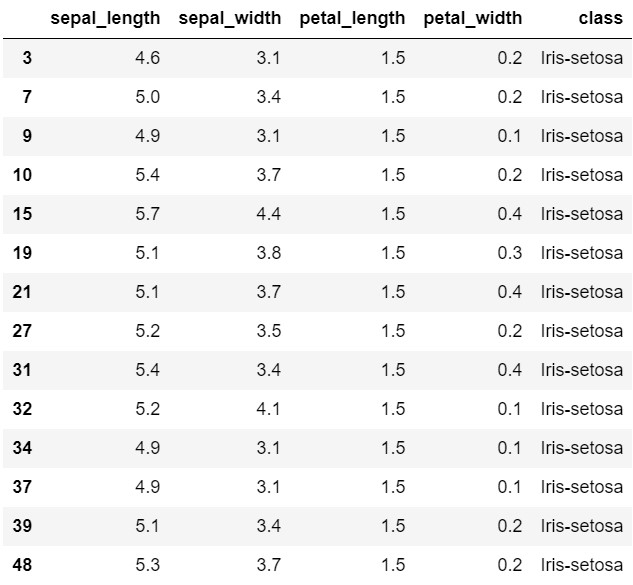
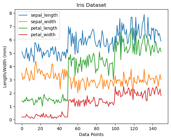
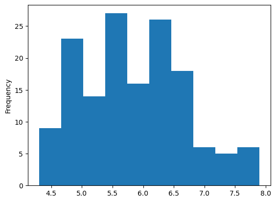
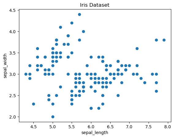
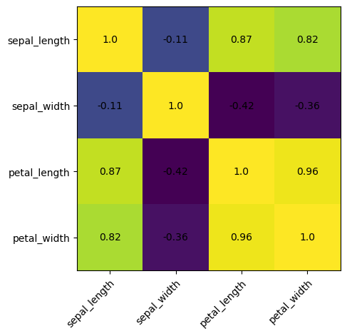
Exhibit 25.59 demonstrates the analysis and visualization of the Iris data using Python’s Pandas and Matplotlib libraries.
Read and View the Iris Dataset
import pandas as pd

# Read data from iris.csv
iris = pd.read_csv('data/iris.csv',
       names=['sepal_length', 'sepal_width', 'petal_length', 'petal_width', 'class'])
print(iris)  # print the first and last five rows of the dataset
     sepal_length  sepal_width  petal_length  petal_width           class
0             5.1          3.5           1.4          0.2     Iris-setosa
1             4.9          3.0           1.4          0.2     Iris-setosa
2             4.7          3.2           1.3          0.2     Iris-setosa
3             4.6          3.1           1.5          0.2     Iris-setosa
4             5.0          3.6           1.4          0.2     Iris-setosa
..            ...          ...           ...          ...             ...
145           6.7          3.0           5.2          2.3  Iris-virginica
146           6.3          2.5           5.0          1.9  Iris-virginica
147           6.5          3.0           5.2          2.0  Iris-virginica
148           6.2          3.4           5.4          2.3  Iris-virginica
149           5.9          3.0           5.1          1.8  Iris-virginica

[150 rows x 5 columns]
Examine the Data’s Structure and Linear Relationship between Fields
# Examine the structure of the dataset
print(iris.shape) # The shape property returns a tuple containing the number of rows and columns of the DataFrame
print(iris.shape[0]) # The number of rows

# correlation to examine the linear relationship between the data fields
iris_new = iris.drop('class', axis=1) # drop column class. axis 0 is row and axis 1 is col
iris_new.corr() # correlation
(150, 5)
150
Filter the Data
# Filter Data
iris[iris['petal_length']==1.5] # filter rows where petal_length is 1.5
Create dataframes iris_setosa, iris_versicolor and iris_virginica
# Create dataframes iris_setosa, iris_versicolor and iris_virginica by filtering the class column
iris_setosa = iris[iris['class']=='Iris-setosa'] # filter iris Setosa
iris_versicolor = iris[iris['class']=='Iris-versicolor'] # filter iris versicolor
iris_virginica = iris[iris['class']=='Iris-virginica'] # filter iris virginica

print(iris_setosa.head(8)) # print top 8 rows
print(iris_versicolor.head(10)) # print top 10 rows
print(iris_virginica.head()) # print top 5 (default value) rows
sepal_length  sepal_width  petal_length  petal_width        class
0           5.1          3.5           1.4          0.2  Iris-setosa
1           4.9          3.0           1.4          0.2  Iris-setosa
2           4.7          3.2           1.3          0.2  Iris-setosa
3           4.6          3.1           1.5          0.2  Iris-setosa
4           5.0          3.6           1.4          0.2  Iris-setosa
5           5.4          3.9           1.7          0.4  Iris-setosa
6           4.6          3.4           1.4          0.3  Iris-setosa
7           5.0          3.4           1.5          0.2  Iris-setosa
    sepal_length  sepal_width  petal_length  petal_width            class
50           7.0          3.2           4.7          1.4  Iris-versicolor
51           6.4          3.2           4.5          1.5  Iris-versicolor
52           6.9          3.1           4.9          1.5  Iris-versicolor
53           5.5          2.3           4.0          1.3  Iris-versicolor
54           6.5          2.8           4.6          1.5  Iris-versicolor
55           5.7          2.8           4.5          1.3  Iris-versicolor
56           6.3          3.3           4.7          1.6  Iris-versicolor
57           4.9          2.4           3.3          1.0  Iris-versicolor
58           6.6          2.9           4.6          1.3  Iris-versicolor
59           5.2          2.7           3.9          1.4  Iris-versicolor
     sepal_length  sepal_width  petal_length  petal_width           class
100           6.3          3.3           6.0          2.5  Iris-virginica
101           5.8          2.7           5.1          1.9  Iris-virginica
102           7.1          3.0           5.9          2.1  Iris-virginica
103           6.3          2.9           5.6          1.8  Iris-virginica
104           6.5          3.0           5.8          2.2  Iris-virginica
Plot the data with Pandas
# default plot is a line chart
ax = iris.plot() # assign to variable ax

# Use ax to add titles and labels
ax.set_title("Iris Dataset")
ax.set_xlabel("Data Points")
ax.set_ylabel("Length/Width (mm)")
Histogram to Examine Sepal Length (with Pandas)
# Histogram
iris["sepal_length"].plot(kind = 'hist') # histogram
Histograms of Iris Species with Matplotlib Subplots
# Matplotlib — for Visualization
import matplotlib.pyplot as plt

# Create subplots with one row and three columns
fig, axes = plt.subplots(nrows=1, ncols=3, figsize=(15, 5))

iris_setosa = iris[iris['class']=='Iris-setosa'] # filter iris Setosa
iris_versicolor = iris[iris['class']=='Iris-versicolor'] # filter iris versicolor
iris_virginica = iris[iris['class']=='Iris-virginica'] # filter iris virginica

# Plot histograms on each subplot
'''
The alpha parameter adjusts the transparency of the elements.
It takes values between 0 (completely transparent) and 1 (completely opaque).
'''
axes[0].hist(iris_setosa["sepal_length"], bins=20, color='blue', alpha=0.7)
axes[0].set_title('Iris Setosa - Sepal Length')
axes[0].set_ylabel('Frequency')

axes[1].hist(iris_versicolor["sepal_length"], bins=20, color='green', alpha=0.7)
axes[1].set_title('Iris Versicolor - Sepal Length')

axes[2].hist(iris_virginica["sepal_length"], bins=20, color='orange', alpha=0.7)
axes[2].set_title('Iris Virginica - Sepal Length')

# Adjust layout to prevent clipping of titles
plt.tight_layout()

# Show the plots
plt.show()
Scatter Plot of the entire Dataset
# creating a scatter plot
# fig: figure. ax: list (array) of subplot
fig, ax = plt.subplots()

# scatter the sepal_length against the sepal_width
ax.scatter(iris['sepal_length'], iris['sepal_width'])
# set a title and labels
ax.set_title('Iris Dataset')
ax.set_xlabel('sepal_length')
ax.set_ylabel('sepal_width')

# Visual examination of the scatter plot reveals 2 or 3 clusters
Scatter Plots and Histograms of the Iris Species
# Subplots of the three species: setosa, virginica, and versicolor
fig, axes = plt.subplots(nrows=2, ncols=3, figsize=(15, 5))

iris_setosa = iris[iris['class']=='Iris-setosa'] # filter iris Setosa
iris_versicolor = iris[iris['class']=='Iris-versicolor'] # filter iris versicolor
iris_virginica = iris[iris['class']=='Iris-virginica'] # filter iris virginica

# First row of charts - histograms
axes[0,0].hist(iris_setosa["sepal_length"], bins=20, color='blue', alpha=0.7)
axes[0,0].set_title('Iris Setosa - Sepal Length')
axes[0,0].set_ylabel('Frequency')

axes[0,1].hist(iris_versicolor["sepal_length"], bins=20, color='green', alpha=0.7)
axes[0,1].set_title('Iris Versicolor - Sepal Length')

axes[0,2].hist(iris_virginica["sepal_length"], bins=20, color='orange', alpha=0.7)
axes[0,2].set_title('Iris Virginica - Sepal Length')

# Second row of charts - scatter plots
axes[1,0].scatter(iris_setosa["sepal_length"], iris_setosa["sepal_width"])
axes[1,0].set_title('Iris Setosa')
axes[1,0].set_xlabel('Sepal Length')
axes[1,0].set_ylabel('Sepal Width')

axes[1,1].scatter(iris_versicolor["sepal_length"], iris_versicolor["sepal_width"])
axes[1,1].set_title('Iris Versicolor')
axes[1,1].set_xlabel('Sepal Length')
axes[1,1].set_ylabel('Sepal Width')

axes[1,2].scatter(iris_virginica["sepal_length"], iris_virginica["sepal_width"])
axes[1,2].set_title('Iris Virginica')
axes[1,2].set_xlabel('Sepal Length')
axes[1,2].set_ylabel('Sepal Width')

# Adjust layout to prevent clipping of titles
plt.tight_layout()

# Show the plots
plt.show()
Heatmap of the Correlation Data
import numpy as np

# Save correlation matrix into variable corr
corr = iris_new.corr()
print(corr)

fig, ax = plt.subplots()

# create heatmap
'''
imshow: is specifically designed to display 2D arrays as images,
    where the color represents the data's magnitude, which fits the
    requirements for visualizing a correlation matrix effectively.
.values: The '.values' attribute returns only the numerical values
    without any row or column labels, in the form of a NumPy array.
'''
ax.imshow(corr.values)
              sepal_length  sepal_width  petal_length  petal_width
sepal_length      1.000000    -0.109369      0.871754     0.817954
sepal_width      -0.109369     1.000000     -0.420516    -0.356544
petal_length      0.871754    -0.420516      1.000000     0.962757
petal_width       0.817954    -0.356544      0.962757     1.000000

Improved Heatmap with Axis Labels and Cell Values
# set labels
'''
arange(): This is a function from the NumPy library that generates an array of evenly
    spaced values within a specified range.
np.arange(start, stop, step): This is the basic syntax though you can omit the start
    and step values to use their defaults (start=0 and step=1).
np.arange(len(corr.columns)): generates an array of integers starting from 0 up to
    (but not including) len(corr.columns).
'''
ax.set_xticks(np.arange(len(corr.columns))) # 'sepal_length', 'sepal_width', 'petal_length', 'petal_width'
ax.set_yticks(np.arange(len(corr.columns))) # 'sepal_length', 'sepal_width', 'petal_length', 'petal_width'
ax.set_xticklabels(corr.columns) # 'sepal_length', 'sepal_width', 'petal_length', 'petal_width'
ax.set_yticklabels(corr.columns) # 'sepal_length', 'sepal_width', 'petal_length', 'petal_width'

# Rotate the tick labels and set their alignment.
plt.setp(ax.get_xticklabels(), rotation=45, ha="right", rotation_mode="anchor")

# Loop over data dimensions to create text annotations.
for i in range(len(corr.columns)): # 'sepal_length', 'sepal_width', 'petal_length', 'petal_width'
    for j in range(len(corr.columns)): # 'sepal_length', 'sepal_width', 'petal_length', 'petal_width'
        # np.around: round by 2 decimal places
        ax.text(j, i, np.around(corr.iloc[i, j], decimals=2),
           ha="center", va="center", color="black")
Exhibit 25.59 Analysis and visualization of the Iris dataset using Python’s Pandas and Matplotlib libraries. Jupyter notebook.
Previous Next
Use the Search Bar to find content on MarketingMind.
Contact | Privacy Statement | Disclaimer: Opinions and views expressed on www.ashokcharan.com are the author’s personal views, and do not represent the official views of the National University of Singapore (NUS) or the NUS Business School | © Copyright 2013-2026 www.ashokcharan.com. All Rights Reserved.


