
-
Sampling
Sampling
Sampling Methods
Simple Random Sampling
Systematic Sampling
Stratified Sampling
Cluster Sampling
Quota Sampling
Convenience Sampling
Purposive Sampling
Snowball Sampling
Mean, Variance, RSE
Sampling Frame
Sample Weighting
Sample Size
Confidence Level, Confidence Interval
Central Limit Theorem
Sample Size — Continuous Parameters
Sample Size — Stratified Sampling
Tracking Studies (Continuous)
Sampling Standards in Retail Measurement
Sample Size — Population Proportions
Subgroups
Tracking Studies
Sample Size — Comparative Studies
Sample and Non-Sample Errors
- Basic Statistics
- Sampling
- Marketing mix Modelling
Coverage Analysis — Retail Measurement Service
- Marketing Education
- Is Marketing Education Fluffy and Weak?
- How to Choose the Right Marketing Simulator
- Self-Learners: Experiential Learning to Adapt to the New Age of Marketing
- Negotiation Skills Training for Retailers, Marketers, Trade Marketers and Category Managers
- Simulators becoming essential Training Platforms
- What they SHOULD TEACH at Business Schools
- Experiential Learning through Marketing Simulators
-
MarketingMind
Sampling
Sampling
Sampling Methods
Simple Random Sampling
Systematic Sampling
Stratified Sampling
Cluster Sampling
Quota Sampling
Convenience Sampling
Purposive Sampling
Snowball Sampling
Mean, Variance, RSE
Sampling Frame
Sample Weighting
Sample Size
Confidence Level, Confidence Interval
Central Limit Theorem
Sample Size — Continuous Parameters
Sample Size — Stratified Sampling
Tracking Studies (Continuous)
Sampling Standards in Retail Measurement
Sample Size — Population Proportions
Subgroups
Tracking Studies
Sample Size — Comparative Studies
Sample and Non-Sample Errors
- Basic Statistics
- Sampling
- Marketing mix Modelling
Coverage Analysis — Retail Measurement Service
- Marketing Education
- Is Marketing Education Fluffy and Weak?
- How to Choose the Right Marketing Simulator
- Self-Learners: Experiential Learning to Adapt to the New Age of Marketing
- Negotiation Skills Training for Retailers, Marketers, Trade Marketers and Category Managers
- Simulators becoming essential Training Platforms
- What they SHOULD TEACH at Business Schools
- Experiential Learning through Marketing Simulators
Sample Size — Population Proportions
When conducting quantitative research, it is common to focus on categorical parameters with discrete values, such as yes/no responses or a 5-point rating scale. These variables follow a binomial distribution, assuming that the population size is sufficiently large.
Typically, interest lies mainly in the proportions. For instance — What proportion of the population are aware of brand X? What proportion of consumers claim they will buy brand X? What proportion of consumers prefer formulation X over formulation Y? What proportion ‘agree’ or ‘strongly agree’ (top 2 boxes) about something?
These variables pertaining to the estimation of a proportion of the population, have two possible outcomes: “success” = 1, “fail” = 0. If the probability of success is p, then:
$$mean, \,µ = p; \,i.e. \,1 × p + 0 × (1-p)$$ $$variance, \,S^2;= p × (1-p)$$Based on the Central Limit Theorem, for a sample size of n, the variance (σ²) of the distribution of sample proportion of successes can be approximated as: $$Variance, \,σ^2= \frac{p(1-p)}{n}$$
The upper bound (maximum value) of sample variance (σ²) is 0.25/n and the upper bound for σ (standard error) is 0.5/√n. This occurs when p=0.5.
Substituting the population variance (S²) in the sample size equation, the required sample size (n) for estimating proportion p̄ is:
$$ n=\frac {Z^2 × p(1-p)}{e^2},\; e = Z \sqrt {\frac {p(1-p)}{n}} $$Where:
- p: is the probability for given response and varies from 0 to 1. It reflects the variability in the data. Note when p=1, (i.e., variance = 0) no sample is required.
- Z: is the standardized value associated with the level of confidence.
- e: is the margin of error.
The probability for which we require the largest sample size is p = 0.5. . Based on this “most conservative” value for p, and for a confidence interval of 95% (Z = 1.96), the required sample size (n) is determined as follows:
Z = 1.96 ≈ 2 for confidence level of 95%
$$p = 0.5$$ $$n = \frac{Z^2p(1-p)}{e^2}≈\frac{2^2×0.5×(1-0.5)}{e^2}$$ $$n≈\frac{1}{e^2},\; e≈\frac{1}{\sqrt n}$$ $$n=\frac{0.96}{e^2},\; e=\frac{0.96}{\sqrt n}$$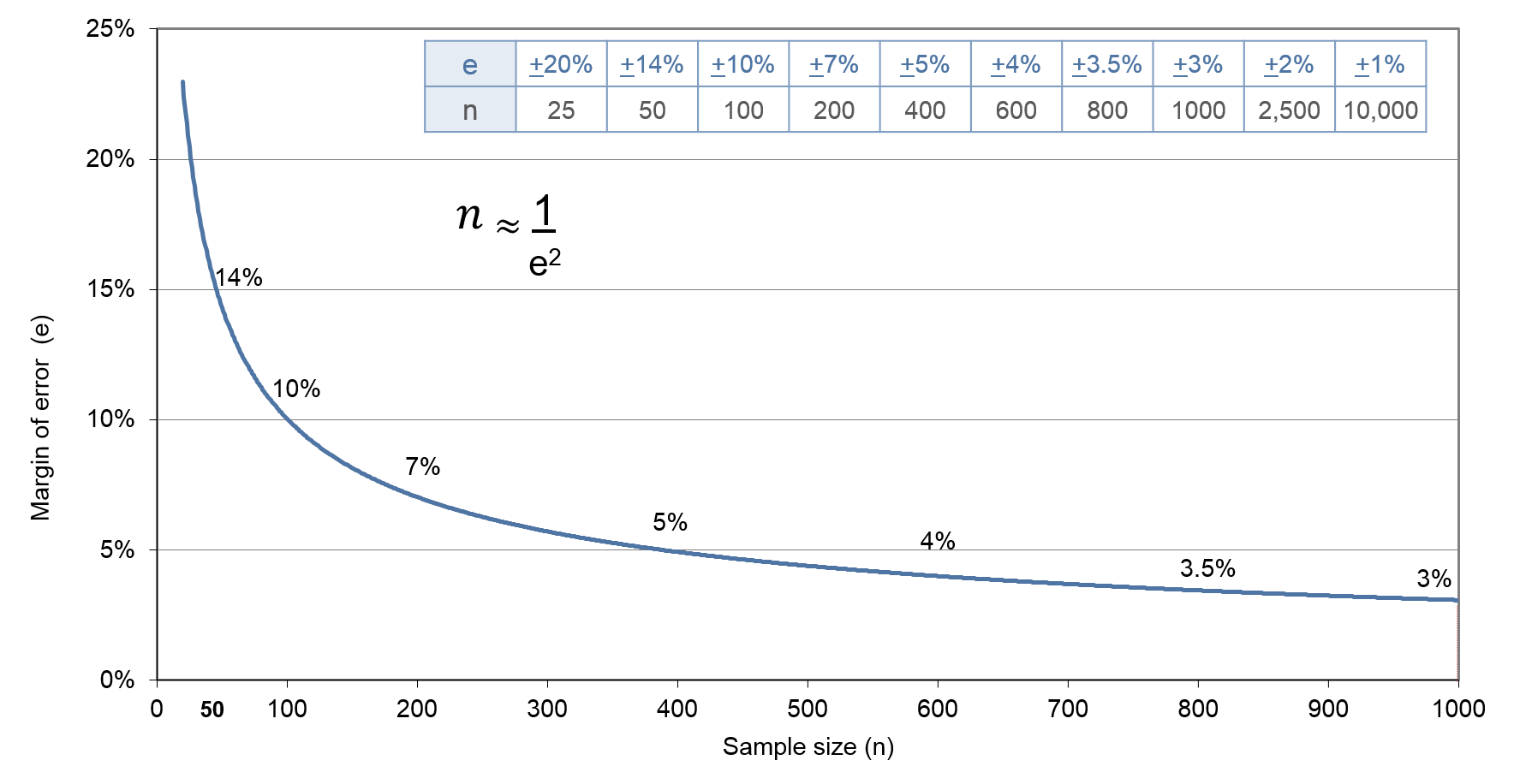
Exhibit 35.3 Estimated sample size required for different margins of error at confidence level of 95%.
Exhibit 35.3 shows how the largest required sample size n varies with the margin of error e. For example, if e = ± 5%, then for the confidence level of 95%, we require a sample of n = 400. Or 384 to be precise if Z (= 1.96) is not rounded off.
Note how the margin of error initially decreases sharply as the sample size, n, increases, and then more gradually. The improvement in accuracy after n=400, is relatively small compared to the increase in sample size.
Example: If 80 respondents out of a sample of 400 consumed a cola drink, we can conclude that 95 times out of 100 (confidence level of 95%), the estimate of the proportion of cola drinkers, over the specified time period, would lie between 16.1% and 23.9% (0.2 ± 0.039):
$$e = 1.96 × \sqrt{0.2(1-0.2)/400}=0.039 $$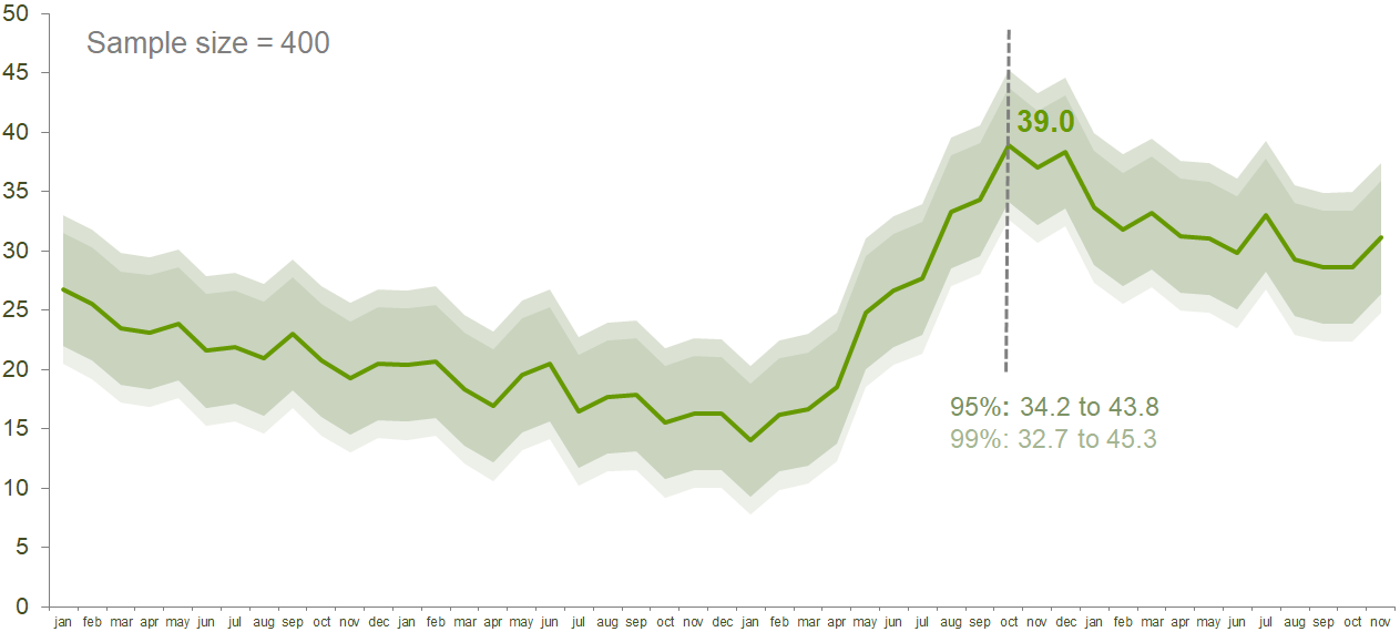
Exhibit 35.4 Dark shaded region depicts the confidence interval for confidence level of 95%. (95% probability that parameter value will lie within this region).
Exhibit 35.4 tracks the results from a monthly study for some parameter along with the confidence interval for confidence levels of 95% (shaded dark) and 99%. The chart tells us that at the peak of 39.0, the confidence interval, taking Z=1.96 and p=0.39, was 34.2% to 43.8%.
The shading in Exhibit 35.4 is a helpful way to visualize the uncertainty in the estimates and to understand the statistical significance of the changes in the parameter. It reveals that while the trend over the years is clearly significant, much of the movement between consecutive months was not statistically significant, even at 95% confidence levels.
Finite Population Correction Factor
In the interest of saving costs, in cases where the universe size is not large, the sample size may be adjusted downwards. For medium size populations, the sample requirement is adjusted downwards using this formula:
$$ n_{adj} = \frac {n}{1+n/N} $$For example, if N = 2000, e = 5% then
$$ n_{adj} = \frac {384}{1+384/1000} $$Additionally, if it is known that the proportions are skewed (i.e., p is not close to 0.5) the sample may be further reduced.
For small universe populations, 100 for instance, it is advisable to take census instead of sample.
Previous Next
Use the Search Bar to find content on MarketingMind.


Contact | Privacy Statement | Disclaimer: Opinions and views expressed on www.ashokcharan.com are the author’s personal views, and do not represent the official views of the National University of Singapore (NUS) or the NUS Business School | © Copyright 2013-2026 www.ashokcharan.com. All Rights Reserved.