-
Marketing mix Modelling
Marketing mix Modelling
Sales Response Function
Linear
Concave
Convex
S-Curve
Interaction Effects
Competitive Effects and Market Share Models
Market Share Models
Dynamic Effects
Adstock
Adfactor
Leads and Lags
Parameter Functions
Long Term Effect (Advertising)
Baseline and Incremental Volume
Promotions Response Model
Model Validity — How Good is the Fit?
Watchouts and Guidelines
Interpretation and Analysis
Discount Elasticity
Cannibalization
Sales Decomposition and Due-To Analysis
What-If Analysis
- Basic Statistics
- Sampling
- Marketing mix Modelling
- Marketing Education
- Is Marketing Education Fluffy and Weak?
- How to Choose the Right Marketing Simulator
- Self-Learners: Experiential Learning to Adapt to the New Age of Marketing
- Negotiation Skills Training for Retailers, Marketers, Trade Marketers and Category Managers
- Simulators becoming essential Training Platforms
- What they SHOULD TEACH at Business Schools
- Experiential Learning through Marketing Simulators
-
MarketingMind
Marketing mix Modelling
Marketing mix Modelling
Sales Response Function
Linear
Concave
Convex
S-Curve
Interaction Effects
Competitive Effects and Market Share Models
Market Share Models
Dynamic Effects
Adstock
Adfactor
Leads and Lags
Parameter Functions
Long Term Effect (Advertising)
Baseline and Incremental Volume
Promotions Response Model
Model Validity — How Good is the Fit?
Watchouts and Guidelines
Interpretation and Analysis
Discount Elasticity
Cannibalization
Sales Decomposition and Due-To Analysis
What-If Analysis
- Basic Statistics
- Sampling
- Marketing mix Modelling
- Marketing Education
- Is Marketing Education Fluffy and Weak?
- How to Choose the Right Marketing Simulator
- Self-Learners: Experiential Learning to Adapt to the New Age of Marketing
- Negotiation Skills Training for Retailers, Marketers, Trade Marketers and Category Managers
- Simulators becoming essential Training Platforms
- What they SHOULD TEACH at Business Schools
- Experiential Learning through Marketing Simulators
Marketing mix Modelling — Dynamic Effects
The impact of some marketing initiatives on sales is often felt not only at the time of the initiative, but also before or after the duration of the initiative. Consumers for instance may respond in anticipation to a price adjustment. Sales may dip after a promotion. Advertising campaigns take time to wear-in, and after they have been aired several times, they begin to wear-out.
The wear-in effect is like an ad that grows on you. Its effectiveness in generating sales increases after consumers are repeatedly exposed to the advertisement, and messages start to register in their minds.
After a prolonged period however, ads start to wear-out. The persuasive impact of advertising, which is important especially for new products, is short term. The repetition of the same message is unlikely to evoke a different response from consumers who are not persuaded to try it. Wear-out also occurs when fatigue sets in — consumers start to get “fed-up” of seeing the same commercial again and again.
Carryover effects may also occur due to various delay factors — consumers’ inter-purchase intervals, delays due to retailer pipeline/lack of adequate stock in trade, delayed consumer response, or the time interval before word-of-mouth effects kick in. These carryover effects tend to be short in duration.
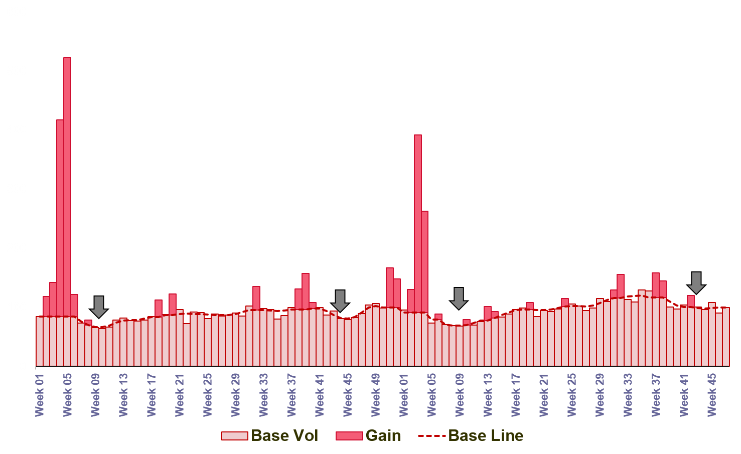
Exhibit 36.3 Take home sales of a FMCG brand reflects dip in sales post festive season as consumers stockpile promoted items.
Promotions are known to impact sales before, during and after the duration of the promotion. In Exhibit 36.3 for example, the sale of a major FMCG item is seen to dip significantly after festive periods. These post promotional losses occur when consumers stockpile goods and are observed after periods of intense festive promotions such as during Christmas or Chinese New Year. A brand may suffer post promotion losses not only when consumers stockpile the brand, but also when consumers stockpile a collection of competing brands. In other word, competitive or interaction effects also come into play.
Over time market dynamics also undergo change. The elasticity of demand for a marketing mix variable can change due to a variety of factors, including the intensity of competition, the magnitude, frequency and recency of prior marketing activities, and various exogenous factors.
All these effects that are spread over time are referred to as dynamic effects. For elements of the marketing mix such as advertising, where the dynamic effects are pronounced, it is important to capture their impact into response models.
Stock Variables — Adstock
One approach to capturing carry over effects is the use of stock variables, adstock for instance. Adstock implicitly distributes the amount of an advertising exposure over several periods. Advertising that is effective at a given time is equal to residual adstock (what is “left over” from previous advertising), plus learning (adstock gained from current advertising). Specifically, if A1, A2, ... At represent the advertising effort (GRP) in periods 1 to t, then the adstock is computed as follows:
$$ Adstock_t=\frac{1-r}{f(1-r)+r}(fA_t+rA_{t-1}+r^2A_{t-2}\, ...\, +r^{t-2}A_2+r^{t-1}A_1),$$ $$A_t=GRP_t.$$Where, r is the retention (or decay) rate, and f (fade) is the impact in the first period. These two parameters may either be pre-fixed by the modeller or determined by the data.
Half-life, the time duration by which the advertising effort has had half its total effect, is a commonly used benchmark for setting f and r.
Advertising Quality — Adfactor
The overwhelming evidence from research studies suggests that the quality of the creative material is critical in advertising. It is important therefore to include advertising quality as a measure when modelling advertising response.
The advertising quality is specific to the commercial, and it may be assessed in terms of consumers’ perception of the advertisement on various measures. One approach used by research firm Millward Brown is based on their Awareness Index (AI). This index is essentially a measure of efficiency of a commercial in generating awareness. It represents the incremental level of claimed ad recall generated per 100 GRPs. An adstock type variable called Adfactor is constructed by using ‘GRP × Awareness Index for the commercial’ as the measure for advertising:
$$ Adfactor_t=\frac{1-r}{f(1-r)+r}(fA_t+rA_{t-1}+r^2A_{t-2}\, ...\, +r^{t-2}A_2+r^{t-1}A_1),$$ $$A_t=AI × GRP_t.$$Where, r is the retention rate, and f is the impact in the first period.
Millward Brown has demonstrated, through practical examples, that incorporating Adfactor into marketing models leads to significantly higher estimates of the contribution of short-term advertising effects.
Leads and Lags
Dynamic promotion effects can also be explicitly modelled by incorporating variables that capture lead and lag effects, i.e.:
$$ S_t=f(X_{t+k}), \, S_t=f(X_{t-k}).$$Commonly used in marketing, the Geometric Distributed Lag (GL) model has a functional form that is structurally similar to that used for stock variables, i.e.:
$$S_t=α+β(1-\lambda)\sum_{l=0}^{\infty}\lambda^l X_{t-l} + \delta_t,\,where\,\delta_t\,is\,the\,disturbance\,term.$$This relation, which is nonlinear, may be converted to a linear estimation model by applying the Koyck transformation:
$$S_t=α+β(1-\lambda)X_t + β(1-\lambda)\sum_{l=1}^{\infty}\lambda^l X_{t-l} + \delta_t $$ $$-\lambda S_{t-1}=-\lambda α - β(1-\lambda)\sum_{l=1}^{\infty}\lambda^l X_{t-l} - \lambda\delta_{t-1} $$ $$S_t-\lambda S_{t-1}=(1-\lambda)α+β(1-\lambda)X_t+(𝛿_t-\lambda 𝛿_{t-1})$$ $$S_t=β_0+β_1X_t+\lambda S_{t-1} + v_t. $$Where vt=𝛿t−λ𝛿t-1, β0=(1−λ)α and β1=(1−λ)β.
In general, for multiple marketing mix variables, the Koyck model becomes:
$$S_t=β_0+\sum_{k=1}^K β_k X_{kt}+\lambda S_{t-1} + v_t $$This model however captures only monotonically decaying carryover effects that do not have a hump. Moreover, estimating the carryovers is tricky when there are multiple independent variables, each with its own carryover effect. Even so the model may provide a fairly good approximation of the underlying response function.
The Autoregressive Distributed Lag Model (ADL) which contains an autoregressive component for sales and a moving average distributed lag component for the mix variables is a general model that captures all types of carryover effects.
$$S_t=β_0+\sum_{p=1}^P \lambda_p S_{t-p} + \sum_{k=1}^K\sum_{q=1}^Q β_{kq} X_{k,t-q}+v_t $$The rate at which the carryover effects peak and decay is controlled by λ, and the number of peaks and their heights is controlled by β.
Parameter Functions
The coefficients of the marketing mix variables in the response models we have discussed so far are assumed to be constant for the analysis period. It is a tenuous assumption considering that many of the dynamic effects imply that these parameters do vary. Parameter functions may be crafted to capture the impact of a variety of these effects, including:
- The magnitude, frequency and recency of prior marketing activities.
- Wear-in and wear-out of advertising.
- Quality of the creative material in advertising.
- Media effects (i.e., differences in ad response due to the choice of TV programme, or section of newspaper).
For instance, consider quality of advertising. We know that effectiveness of advertising is dependent greatly on the creative material. One approach to capturing this effect is by means of a variable that captures both quantity and quality, the Adfactor for instance. We could also capture the ad quality effect by means of a process function for the advertising coefficient, i.e., βadvt=f(ad campaign).
Similarly, the price-promotion elasticity (discount elasticity) of products can change due to the magnitude and frequency of previous discounts. If heavy promotions are repeated too frequently, their impact begins to fade. Frequent, attractive promotions also tend to induce an opportunistic behaviour — consumers lie in wait for the deals, resulting in the lowering of the base line. The parameters for price discount, promotion (e.g., display, co-op advertising) and baseline (i.e., store intercept) are therefore a function of historical levels of promotions.
One approach to capturing the dynamic nature of the market is by means of multistage models where the coefficients of the mix variables estimated at the first stage become the dependent variable in the next stage. In the second stage, where the coefficients of the mix variables are treated as the dependent variables, the independent variables are the characteristics that influence the coefficient.
Previous Next
Use the Search Bar to find content on MarketingMind.
Contact | Privacy Statement | Disclaimer: Opinions and views expressed on www.ashokcharan.com are the author’s personal views, and do not represent the official views of the National University of Singapore (NUS) or the NUS Business School | © Copyright 2013-2026 www.ashokcharan.com. All Rights Reserved.

