Coverage Analysis — Retail Measurement Service

NOTE: This article which pertains to consumer marketing assumes familiarity with retail tracking services. It is sourced from the Marketing Analytics Practitioner's Guide

Several years back, a brand manager pompously threw a report on the table, proclaiming it was “utter rubbish”.

Though usually not so blunt, similar sentiments are often expressed as marketers struggle to bridge the void between the theoretical concepts taught in schools and the practical knowledge and understanding that is required in the industry.

ORG-MARG’s coverage was only 40-50% of sales of Hindustan Lever’s brands in 1992. Provided he understands what is covered and what is not covered, the brand manager can make very good use of the data.

Contents

Coverage Gap
Coverage varies from Item to Item
Revealing and Misleading
Coverage Analysis
What use is a report that does not reflect my entire market?

Coverage Gap

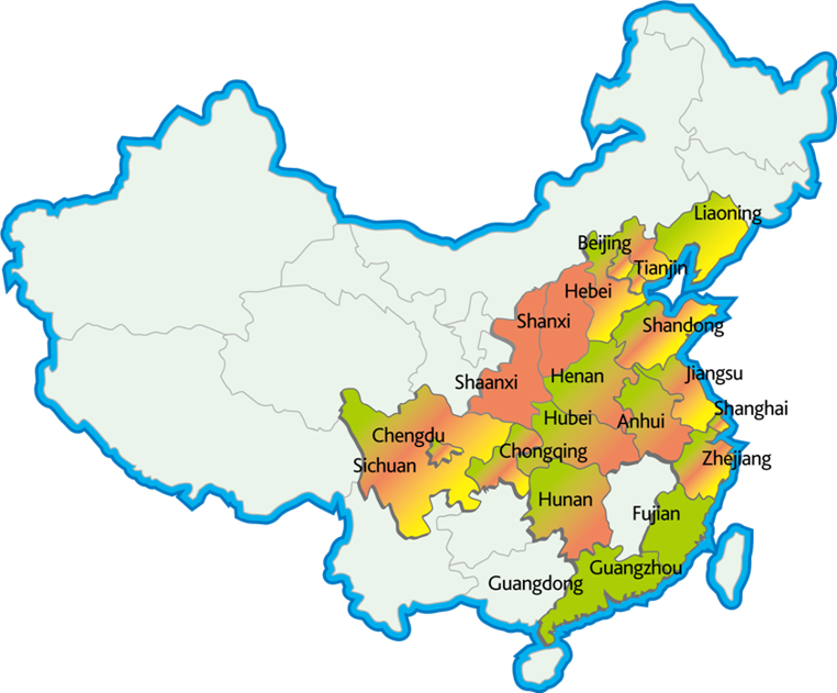
Exhibit 20.14 Nielsen’s RMS covers the more densely populated urban provinces of China.

The retail measurement service (RMS) tracks the sales of goods from retailers to consumers, at specific outlets in a predefined geographical area referred to as the retail universe. This universe is usually not the same as the supplier’s sales territory. For example in China (Exhibit 20.14), the Nielsen RMS covers the densely populated urban provinces of China, leaving out the sparsely populated regions in the West.

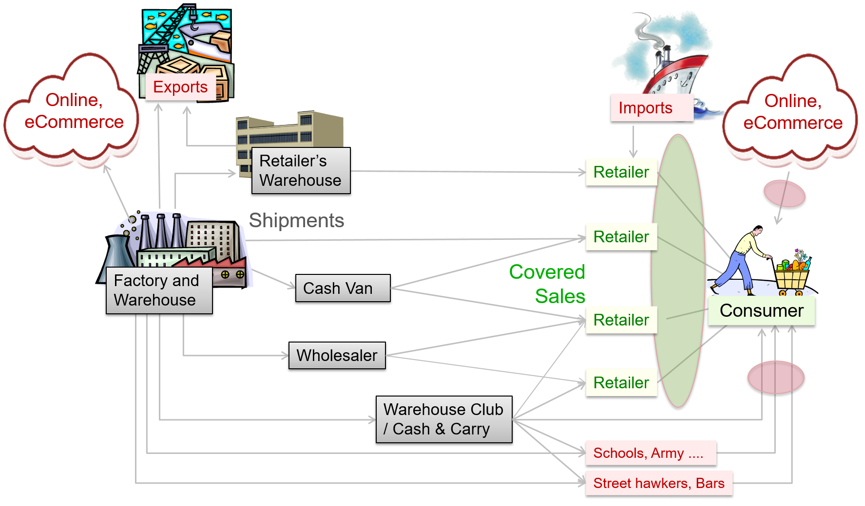
Exhibit 20.15 Distribution network, shipments and covered sales.

Moreover, as depicted in Exhibit 20.15, within the same geographical boundaries, the supplier may sell to outlets at locations such as schools and military establishments that are not accessible to the RMS service provider. There are several such outlets that are not accessed by the service including the few listed here:

Chain of hotels not willing to co-operate with the service provider.
Retail outlets selling cigarettes at construction sites where entry is restricted.
Outlets at tourist locations that usually sell large quantities of impulse products like ice cream and chocolates. It may not be viable for the service provider to access these stores.

Outlets such as these are the prime reason for the existence of what is referred to as the coverage gap.

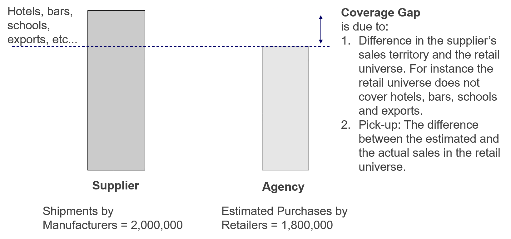
Exhibit 20.16 Coverage gap is the shortfall between the agency’s estimated purchases by retailers and the manufacturer’s shipments.

As shown in Exhibit 20.16, the difference between the supplier’s shipments and agency’s estimate of store purchases is the coverage gap. This gap arises due to the following reasons:

As mentioned above, the retail universe is not the same as the supplier’s sales territory.
The pipeline, or specifically the increase or decrease of stocks within it. The pipeline comprises of all the intermediate locations that items pass on their journey from the supplier’s warehouse to the consumer’s shopping cart. Due to its existence, there is a time lag from the moment an item is shipped from the supplier’s warehouse to the instance it is bought by a consumer.
Export and imports or parallels as they are often referred to. If parallels constitute a large component of goods sold in the retail universe, as is the case for some brands of bar soaps in Singapore, then coverage may exceed 100%.
Inaccuracies in the agency’s estimates, arising due to sampling and other factors pertaining to method of tracking sales. This is referred to as pick-up error.

The build-up or depletion of the pipeline inventory significantly affects the coverage gap. These fluctuations occur due to several factors some of which are listed below:

Irregular shipment patterns; which can arise when there is a change in the intermediaries. For instance when new distributors are appointed.
Investment buying by retailers. This occurs when suppliers offer high trade discounts that result in fluctuations in the pipeline flow.
Trade and consumer promotions also influence stock levels within the pipeline.
Longevity of a product. Goods such as bread, pasteurized milk that have short lives are likely to have shorter pipelines, and they pass much more quickly from factory to retail store. In the case bread for instance, most manufacturers deliver directly to retail outlets on a daily basis.
Distribution network. An elaborate structure of wholesalers, agents, distributors and concessionaires lengthens the pipeline effect.
Geography or more specifically the size of the sales territory. Larger countries require more elaborate distribution networks to service the entire sales territory.
Coverage also varies over the life cycle of product, as can be seen from Exhibit 20.17. This is covered in more detail in the next section.

Coverage varies from Item to Item

For a variety of reasons, the coverage of some items is better than that for others. Items within the same market breakdown and even items within the same product category can have markedly different coverage levels.

Some of the reasons for this have been stated earlier. The longevity of a product for instance has a bearing on the length of the pipeline and the amount of stocks in the pipeline, which affects the coverage.

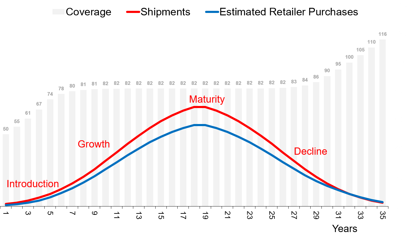
Exhibit 20.17 Coverage varies over a product’s life cycle, particularly during its introduction and decline. (As there are many other factors affecting it, coverage will fluctuate more widely than shown above).

Coverage also varies over the product’s life cycle. As can be seen from Exhibit 20.17, when a product is introduced, stocks starts to fill the pipeline as they move from the supplier to retail outlets. While the pipeline expands, retailer purchases grow at a slower pace than shipments, and coverage is below norm. When the pipeline fills up and the expansion of the distribution network starts to level off, coverage starts to stabilize. (Due to other factors, it is never as stable as depicted in the exhibit).

Later on when the product is in decline, the pipeline starts to shrink, and pipeline inventories decline sharply. Over these years, shipments are lower than retailer purchases, and this raises the coverage level.

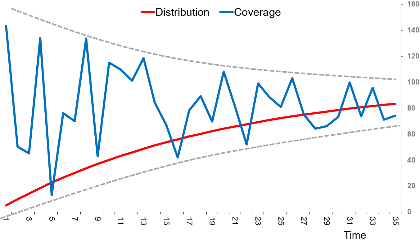
Exhibit 20.18 Product’s distribution level affects the accuracy of sales and purchases estimates.

The accuracy of the purchases and sales estimates is affected by the level of distribution of a product. When the distribution is low, the number of stores stocking the product in the agency’s sample of retail outlets is small. As distribution expands, it is found in more stores in the agency’s sample. The resulting increase in the effective sample size improves the accuracy of the purchases and sales estimates. As can be seen from Exhibit 20.18, this greatly reduces the volatility in coverage estimates.

Revealing and Concealing

RMS data is usually very revealing. At times, however, it can also be misleading. Which is why it is important to fully appreciate the strengths and limitations of the service, particularly in the context of coverage.

Thorough knowledge of the structure and methodology builds greater confidence in the service, and imparts an improved understanding of the data.

The data is usually well received, if it is good news. It is more revealing, though, when the news is not as expected, and that is when manufacturers need to be prepared to “listen” to what the data is saying.

Here are a few examples that illustrate the point.

Kraft Builder — Indonesia

In the last quarter of 2007, a few years after they took over Danone’s biscuits business, Kraft Indonesia changed their distribution network. The previous network relied on one national distributor, encompassing 26 branches and 28 sub-districts. The new distribution network, named Builder, relied on 15 territory level distributors, encompassing 39 branches and 13 sub-districts.

Kraft estimated that retailer coverage increased from 87,000 (pre-Builder) to 165,000 stores, by end 2007.

The company’s shipments of biscuits surged by roughly 40% in 2008. This seemed like a huge success … it was one of the reasons CEO, Irene Rosenfeld, made it a point to meet the Indonesian team on her visit to the Asia Pacific region.

The only dampener was that estimates by Nielsen Indonesia showed substantially lower increase in sales. At that time is was hard to accept the Nielsen data.

In 2009, when Kraft’s biscuits shipments plunged it confirmed what one should have inferred from the start.

The key reason for the surge in sales in 2008 was the development of the parallel sales pipeline. The new Builder distribution network was significantly larger, and importantly, the depletion of stocks in the old pipeline was occurring at a far slower pace than the build-up in the new one.

As a result, a large proportion of the 40% increase in sales was due to the increase in the pipeline inventory, which for a big country like Indonesia can be quite large. When the expansion of the Builder distribution network levelled off, the temporary excess of stocks in trade due to the continued existence of the old network, parallel to the new one, resulted in the plunge in the shipments in 2009.

Shipments stabilized when stocks in the old distribution network depleted and the network ceased to exist.

During the transition years, while shipments jumped up and down like a yoyo, the Nielsen sales estimates grew at a steady pace. The turbulence in the intermediary networks did not have an adverse effect on consumer offtake.

Investment Buying

Investment buying can cause confusion.

Some years back, when the channel was still more significant, Organic shampoo shipments to provision stores in Singapore surged from an average of 17 thousand litres to 53 thousand litres. This was primarily the outcome of a trade promotion, and though retailer purchases reflected a small increase, consumer purchases remained flat.

In this case, distributors where happy to stock up thus inflating the pipeline and because they did not pass any of the discounts they received to retailers or the consumers, there was no incentive for them to purchase more than their usual requirement.

In another example, a western soup manufacturer sold extraordinarily large quantities of canned soup to a dominant supermarket chain by offering a large trade discount. Subsequently the manufacturer’s country head was so disappointed with the sales reports that he discontinued subscribing to the RMS service.

Yet it takes both push and pull to lift consumer purchases. And eating habits are hard to change.

Even if the incentive given to the supermarket was passed onto consumers, it would have been difficult to entice a population that is predominantly ethnic Chinese, to increase their purchases of western canned soup.

If the aim was to sell beyond a small segment to the larger market, the manufacturer needed to develop varieties that appealed to the senses, preferences and tastes of that market. Which is easier said than done.

Abbott Laboratories — Malaysia

As mentioned earlier, though it is usually revealing, RMS data can also be misleading.

Abbott Laboratories, the manufacturers of infant formula, substantially increased their sales in Malaysia by expanding into newer channels of distribution. Unfortunately, for the Abbott team, these channels were not covered by Nielsen Malaysia, and so, it turned out that the Nielsen data reflected a decline in sales.

The decline was because, in addition to growing Abbott’s overall business, there was some cannibalization of the established channels covered by Nielsen Malaysia, by the new channels not covered by the agency.

Nielsen’s market share was a KPI for Abbott, and despite a written explanation, the global Abbott management made no exception for the Malaysian team.

Coverage Analysis

The above illustrations highlight the importance of knowing the strengths and limitations of the retail measurement service, and understanding the dynamics of primary, secondary and tertiary sales.

Coverage analysis is an important exercise that helps the agency and its clients assess the coverage gap. This information is used by the agency to prioritize improvements to their service. It also helps the clients in their interpretation of the data.

Coverage analysis is based on moving annual totals (MAT) of reported retailer purchases and manufacturer’s shipments. It relies on three parameters:

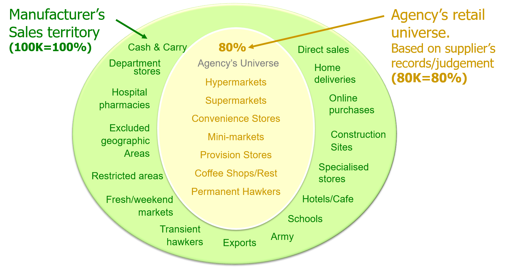
Coverage: The agency’s estimated retailer purchase volume as a percentage of supplier’s shipments.
Expected Coverage: The proportion of supplier’s total shipments that go to the retail universe. This is based on supplier’s records and their judgement.
Pick Up: The agency’s estimated retailer purchase volume as a percentage of supplier’s shipments that go to the retail universe.

As may be gauged from the above definitions:

Coverage = Expected Coverage × Pick Up

Coverage reflects the extent to which the RMS estimates relate to the supplier’s shipment. It is a measure of the accuracy of the service as a whole and is dependent on the extent to which the retail universe captures the manufacturer’s shipments (expected coverage) as well as the accuracy of the research methodology (pick up).

Pick up is a measure of the accuracy of the research methodology and is dependent on the sampling framework as well as non-sampling errors.

Exhibit 20.19 Expected coverage is the proportion of supplier’s total shipments that go to the retail universe. In this example, based on sales records and judgement, the manufacturer estimates that 80% of total shipments go through the outlets covered by the agency.

Example (see Exhibit 20.19):

Total Shipments = 100 thousand units. (Supplier’s shipments of product in the sales territory is 100 thousand units).
Shipments into Retail Universe = 80 thousand units. (Based on sales records and judgement, the manufacturer estimates that 80 thousand units were sold to the retailers covered by the agency).
Expected Coverage = 80K/100K = 80%. (The proportion of supplier’s total shipments that go to the retail universe).
Retailer Purchases = 72 thousand unit. (The agency’s estimated retailer purchase volume of the product).
Pick Up = 72K/80K = 90%. (The agency’s estimated retailer purchase volume as a percentage of supplier’s shipments that go to the retail universe).
Coverage = 72K/100K = 72% = Expected Coverage × Pick Up
(The agency’s estimated retailer purchase volume as a percentage of supplier’s shipments).

Coverage analysis is conducted on moving annual totals (MAT). This limits pipeline effect, i.e., the lag between the time of shipment of goods from the factory and the time the goods reach the retailer. It also smoothens out the impact of promotions and seasonality.

Moreover, compared to consumer offtake, manufacturer’s shipments tend to be volatile with peaks and troughs over months. The yearly totals even out these variances.

The sales territory in a coverage analysis should represent the total country. This reduces errors due to cross-country movement of goods.

Note also that coverage analysis is appropriate for brands with numeric distribution of 80% or above. This conforms with Nielsen’s global standard for sampling error, which applies to products that are available in 80% of the universe. Estimates for products with lower levels of distribution may not meet the agency’s global norms.

Manufacturers should review coverage for major brands once in every two to three years, or more frequently if there is are concerns regarding the quality of the data. At the agency, the measurement scientists (or data scientists as they are now called) should be conducting the analysis on a regular basis as it provides critical information on the how their service can be enhanced.

Reverting to our example, 90% pick up is good.

Whether expected coverage of 80% is good depends on several factors. While it is usually not practical or viable to achieve full coverage, opportunities to improve, as and when they arise, should be exploited.

What is more important is that, unless there are compelling reasons, the average coverage levels should not fall. The retail environment is constantly changing, and it is important that the RMS service continually adapts so that high standard are maintained.

What use is a report that does not reflect my entire market?

A market research/analytics report is not a financial statement. In order to understand market forces, it is not critical that the dollars and cents add up.

A major reason why the numbers do not add up is because coverage is rarely 100% — some distribution channels are either too difficult or too expensive to track. Since they can only rely on what they have, marketers need to understand the strengths and limitations of the data.

Retail tracking data reveals information pertaining only to the channels that are covered. Provided coverage levels are not too low, this information imparts a good understanding of the underlying market trends. However, care needs to be taken with interpretations when market dynamics differ substantially between the areas that are covered and those that are not.

Take for instance the Abbott example cited earlier. If outlets in the areas that are excluded from coverage are cannibalizing those that are included, the data will not reveal this important underlying trend.

For a deeper understanding of market dynamics, marketer should rely on multiple data sources. As discussed in the section Interpretation and Recommendation, in Chapter Quantitative Research, firmer conclusions are formed by triangulating data. A single source often raises questions (why are sales declining?), and opens up possibilities (is it due to price? Competition? Distribution?). Piecing together the facts from diverse data sources yields deeper understanding of the market dynamics.

Nov 22, 2017: Dollars, digits and data: The disruption of marketing
Oct 26, 2017: How dollars, digits and data are transforming marketing
Sep 25, 2017: Disrupting marketing: Tech and the business of selling
May 28, 2017: Coverage Analysis — Retail Measurement Service
May 25, 2017: Time for Singapore Airlines to bring back the Magic
May 19, 2017: Infant Milk — The Real Reasons why Prices Soared, and the Lesson for Marketers
May 5, 2017: Dove Bottle Ad — Commentary
April 12, 2017: Social Cloisters and Fake News